Matlab中的网格检测

15

我有一张二进制图像中的网格(可能会旋转)。如何使用MATLAB知道该网格的近似公式?

示例图像:


(来源: sjtu.edu.cn)

有时这些黑点会丢失,因此我需要一个公式或“方法”来估计这些黑点可能的中心。

我已尝试使用regionprops,它可以帮助我获取存在的黑点的中心,但不知道如果缺少黑点,则无法估计。

clear all
im = imread('print5.jpg');
im = im2bw(im);
[sy,sx] = size(im);
im = imcomplement(im);
im(150:200,100:150) = 0; % let some dots missing!
im = imclearborder(im);
st = regionprops(im, 'Centroid');

imshow(im) hold on;
for j = 1:numel(st)
    px = round(st(j).Centroid(1,1));
    py = round(st(j).Centroid(1,2));
    plot(px,py,'b+')
end

1
尝试查看频率内容:fft2 网格非常规则,您应该能够在频率域中发现峰值。 - Shai
5
如果你将上述评论中的所有信息编辑到你的问题中,那么你应该能够重新打开它。 - Paul R
5
哇,这个在短时间内吸引了很多负评。我理解为什么它会被关闭,但它真的值得受到-20的负评吗? - Amro
3
如果您查看主页,您会发现问题已经超过一个小时没有更新了,这可能是他们这样做的原因。通常,被投票为-3 / -4 的问题会从“最新问题”部分中移除,以防止进一步的投票,但由于这个故障,这个问题仍然显示出来 :/。 - dsgriffin
3
我已经添加了原帖作者的代码和评论描述。这应该会减缓那些盲目点踩的人。如果你是其中之一,请重新考虑一下。 - Amro
显示剩余2条评论
2个回答

41

以下是一种使用fft在x和y投影上进行1D处理的方法:

首先,我会通过与高斯卷积来模糊图像以消除高频噪声:

m=double(imread('print5.jpg'));
m=abs(m-max(m(:))); % optional line if you want to look on the black square as "signal"
H=fspecial('gaussian',7,1);
m2=conv2(m,H,'same');

然后我将对每个轴的投影进行fft:

delta=1;
N=size(m,1);
df=1/(N*delta);        % the frequency resolution (df=1/max_T)
f_vector= df*((1:N)-1-N/2);     % frequency vector 

freq_vec=f_vector;
fft_vecx=fftshift(fft(sum(m2)));
fft_vecy=fftshift(fft(sum(m2')));
plot(freq_vec,abs(fft_vecx),freq_vec,abs(fft_vecy))

在这里输入图片描述

我们可以看到两个轴都在0.07422处达到峰值,这相当于1/0.07422像素或约13.5像素的周期。

获取角度信息的更好方法是进行二维计算,即:

ml= log( abs( fftshift (fft2(m2)))+1);
imagesc(ml) 
colormap(bone)

在此输入图像描述

然后,如果需要,可以使用简单的几何形状或regionprops等工具来获取正方形的角度和大小。正方形的大小是背景上大正方形的大小的1/(因为我模糊了图像,所以可能有些模糊,请努力不要这样做),而角度则是atan(y/x)。正方形之间的距离是中心部分到图像中心处强峰之间距离的1/。

因此,如果适当地阈值化ml图像,则会得到:

 imagesc(ml>11)

你可以访问中心峰以实现这个目标...

另一种方法是对二进制图像进行形态学操作,例如阈值化模糊图像并将对象缩小为点。它会去除像素,使没有孔的对象缩小到一个点:

BW=m2>100;
BW2 = bwmorph(BW,'shrink',Inf);
figure, imshow(BW2)

在此输入图像描述

那么你实际上有一个每个晶格点一个像素的网格!因此,您可以使用霍夫变换将其馈送给Amro's solution,或者进行fft分析,或适合于块等...


28
您可以应用
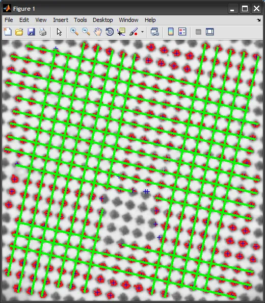
霍夫变换来检测网格线。一旦我们有了这些,您就可以推断出网格位置和旋转角度:
%# load image, and process it
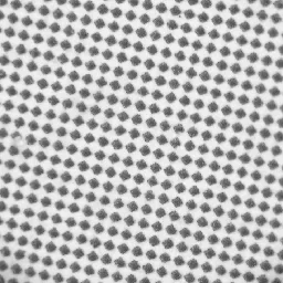
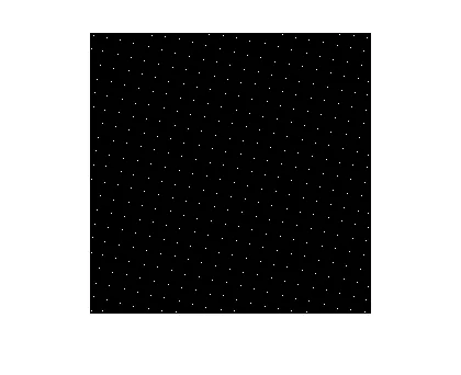
img = imread('print5.jpg');
img = imfilter(img, fspecial('gaussian',7,1));
BW = imcomplement(im2bw(img));
BW = imclearborder(BW);
BW(150:200,100:150) = 0;    %# simulate a missing chunk!

%# detect dots centers
st = regionprops(BW, 'Centroid');
c = vertcat(st.Centroid);

%# hough transform, detect peaks, then get lines segments
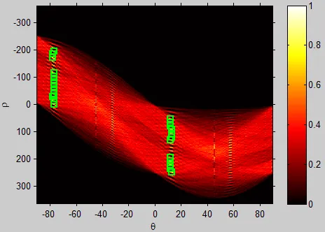
[H,T,R] = hough(BW);
P  = houghpeaks(H, 25);
L = houghlines(BW, T, R, P);

%# show image with overlayed connected components, their centers + detected lines
I = imoverlay(img, BW, [0.9 0.1 0.1]);
imshow(I, 'InitialMag',200, 'Border','tight'), hold on
line(c(:,1), c(:,2), 'LineStyle','none', 'Marker','+', 'Color','b')
for k = 1:length(L)
    xy = [L(k).point1; L(k).point2];
    plot(xy(:,1), xy(:,2), 'g-', 'LineWidth',2);
end
hold off

我正在使用来自文件交换的 imoverlay 函数。
结果如下:

grid_lines_overlayed

这是累加器矩阵,对应检测到的直线峰值已经标出:

accumulator_peaks


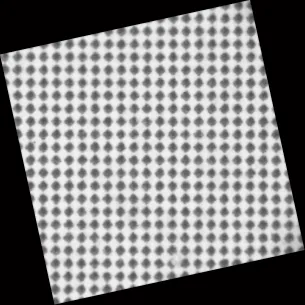
现在,我们可以通过计算检测到的线条的平均斜率来恢复旋转角度,过滤掉不是水平或垂直方向的线条。
%# filter lines to extract almost vertical ones
%# Note that theta range is (-90:89), angle = theta + 90
LL = L( abs([L.theta]) < 30 );

%# compute the mean slope of those lines
slopes = vertcat(LL.point2) - vertcat(LL.point1);
slopes = atan2(slopes(:,2),slopes(:,1));
r = mean(slopes);

%# transform image by applying the inverse of the rotation
tform = maketform('affine', [cos(r) sin(r) 0; -sin(r) cos(r) 0; 0 0 1]);
img_align = imtransform(img, fliptform(tform));
imshow(img_align)

这里是将图像旋转回来,使得网格与xy轴对齐的结果:
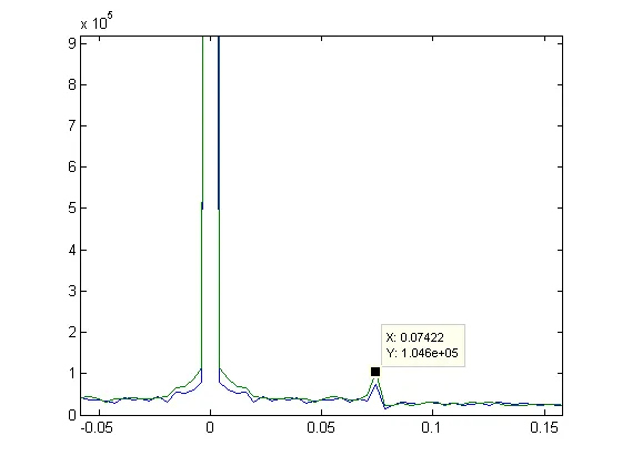
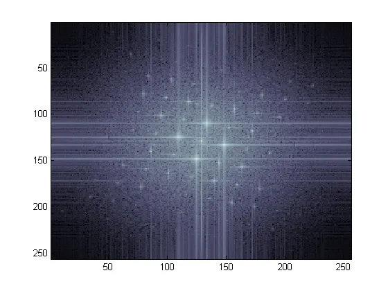
aligned_img


网页内容由stack overflow 提供, 点击上面的
可以查看英文原文,
原文链接