Matlab中的螺旋网格

Question

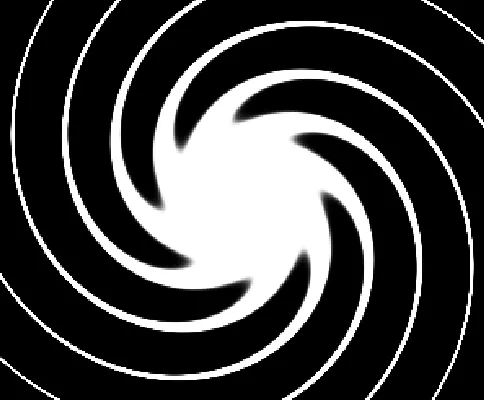
我正在尝试使用MATLAB生成一些计算机生成的全息图。我使用等间距网格初始化空间网格，并获得了以下图像。

这种图案有点符合我的需求，除了中心区域。条纹应该是锐利但模糊的。我认为这可能是网格的问题。我尝试在极坐标下生成网格，然后使用MATLAB的pol2cart函数将其映射到笛卡尔坐标中。不幸的是，它效果并不好。有人建议使用细网格。这也行不通。我认为如果我能生成一个螺旋网格，也许问题就可以解决。此外，螺旋臂的数量通常是任意的，有人能给我一些提示吗？

我附上了代码（我的最终项目并不完全相同，但存在类似的问题）。

clc; clear all; close all;
%% initialization
tic
lambda = 1.55e-6;
k0 = 2*pi/lambda;
c0 = 3e8;
eta0 = 377;
scale = 0.25e-6;
NELEMENTS = 1600;
GoldenRatio = (1+sqrt(5))/2;
g = 2*pi*(1-1/GoldenRatio);

pntsrc = zeros(NELEMENTS, 3);
phisrc = zeros(NELEMENTS, 1);
for idxe = 1:NELEMENTS
  pntsrc(idxe, :) = scale*sqrt(idxe)*[cos(idxe*g), sin(idxe*g), 0];
  phisrc(idxe) = angle(-sin(idxe*g)+1i*cos(idxe*g));
end
phisrc = 3*phisrc/2; % 3 arms (topological charge ell=3)

%% post processing
sigma = 1;
polfilter = [0, 0, 1i*sigma; 0, 0, -1; -1i*sigma, 1, 0]; % cp filter

xboundl = -100e-6; xboundu = 100e-6;
yboundl = -100e-6; yboundu = 100e-6;
xf = linspace(xboundl, xboundu, 100);
yf = linspace(yboundl, yboundu, 100);
zf = -400e-6;
[pntobsx, pntobsy] = meshgrid(xf, yf);
% how to generate a right mesh grid such that we can generate a decent result?
pntobs = [pntobsx(:), pntobsy(:), zf*ones(size(pntobsx(:)))];
% arbitrary mesh may result in "wrong" results

NPNTOBS = size(pntobs, 1);
nxp = length(xf);
nyp = length(yf);

%% observation
Eobs = zeros(NPNTOBS, 3);

matlabpool open local 12
parfor nobs = 1:NPNTOBS
  rp = pntobs(nobs, :);
  Erad = [0; 0; 0];
  for idx = 1:NELEMENTS
    rs = pntsrc(idx, :);
    p = exp(sigma*1i*2*phisrc(idx))*[1 -sigma*1i 0]/2; % simplified here
    u = rp - rs;
    r = sqrt(u(1)^2+u(2)^2+u(3)^2); %norm(u);
    u = u/r; % unit vector
    ut = [u(2)*p(3)-u(3)*p(2),...
      u(3)*p(1)-u(1)*p(3), ...
      u(1)*p(2)-u(2)*p(1)]; % cross product: u cross p
    Erad = Erad + ... % u cross p cross u, do not use the built-in func
      c0*k0^2/4/pi*exp(1i*k0*r)/r*eta0*...
      [ut(2)*u(3)-ut(3)*u(2);...
      ut(3)*u(1)-ut(1)*u(3); ...
      ut(1)*u(2)-ut(2)*u(1)]; 
  end
  Eobs(nobs, :) = Erad; % filter neglected here
end
matlabpool close
Eobs = Eobs/max(max(sum(abs(Eobs), 2))); % normailized

%% source, gaussian beam
E0 = 1;
w0 = 80e-6;
theta = 0; % may be titled
RotateX = [1, 0, 0; ...
  0, cosd(theta), -sind(theta); ...
  0, sind(theta), cosd(theta)];

Esrc = zeros(NPNTOBS, 3);
for nobs = 1:NPNTOBS
  rp = RotateX*[pntobs(nobs, 1:2).'; 0];
  z = rp(3);
  r = sqrt(sum(abs(rp(1:2)).^2));
  zR = pi*w0^2/lambda;
  wz = w0*sqrt(1+z^2/zR^2);
  Rz = z^2+zR^2;
  zetaz = atan(z/zR);
  gaussian = E0*w0/wz*exp(-r^2/wz^2-1i*k0*z-1i*k0*0*r^2/Rz/2+1i*zetaz);% ...
  Esrc(nobs, :) = (polfilter*gaussian*[1; -1i; 0]).'/sqrt(2)/2;
end
Esrc = [Esrc(:, 2), Esrc(:, 3), Esrc(:, 1)];
Esrc = Esrc/max(max(sum(abs(Esrc), 2)));  % normailized
toc

%% visualization
fringe = Eobs + Esrc; % I'll have a different formula in my code
normEsrc = reshape(sum(abs(Esrc).^2, 2), [nyp nxp]);
normEobs = reshape(sum(abs(Eobs).^2, 2), [nyp nxp]);
normFringe = reshape(sum(abs(fringe).^2, 2), [nyp nxp]);

close all;
xf0 = linspace(xboundl, xboundu, 500);
yf0 = linspace(yboundl, yboundu, 500);
[xfi, yfi] = meshgrid(xf0, yf0);
data = interp2(xf, yf, normFringe, xfi, yfi);
figure; surf(xfi, yfi, data,'edgecolor','none');
% tri = delaunay(xfi, yfi); trisurf(tri, xfi, yfi, data, 'edgecolor','none');
xlim([xboundl, xboundu])
ylim([yboundl, yboundu])
% colorbar
view(0,90)
colormap(hot)
axis equal
axis off
title('fringe thereo. ', ...
  'fontsize', 18)

- Tony Dong

---

我不确定……我认为你可能已经是任意武装螺旋网格的专家了。但如果你找到答案，请告诉我们——世界需要更多像这样的螺旋体。 - pancake

我无法以高效的方式生成螺旋网格，并且这里的图形确实不准确。 - Tony Dong

请展示您的代码，以便我们了解为什么会发生这种情况。 - bla

我已经附上了部分代码。 - Tony Dong

我明白了。但是你建议的并不完全符合我的需求。正如你所说，如果我应用喷气式颜色映射，我会得到很多模糊，表明边缘本质上是锐利的。（实际上确实如此。）我认为中心区域的幅度应该更高。如果是这样，无论我们使用什么类型的颜色函数，我们都可以在中间获得较少模糊的漂亮边缘。 - Tony Dong

Answer 1

我没有阅读你的代码，因为它太长了，而且做这样一个简单的事情。我写了我的代码，这是结果：

代码是

%spiral.m
function val = spiral(x,y)

  r = sqrt( x*x + y*y);
  a = atan2(y,x)*2+r;                  

  x = r*cos(a);
  y = r*sin(a);

  val = exp(-x*x*y*y);

   val = 1/(1+exp(-1000*(val)));   

endfunction


%show.m
n=300;
l = 7;
A = zeros(n);

for i=1:n
for j=1:n
    A(i,j) = spiral( 2*(i/n-0.5)*l,2*(j/n-0.5)*l);
end
 end


imshow(A) %don't know if imshow is in matlab. I used octave.

锐度的关键在于线条。

val = 1/(1+exp(-1000*(val))); 

这是逻辑函数。数字1000定义了图像的清晰度，因此将其降低可获得更模糊的图像，将其提高可获得更清晰的图像。

希望这回答了你的问题 ;)

编辑：玩起来真有趣。这是另一个螺旋图案：

function val = spiral(x,y)

   s= 0.5;

   r = sqrt( x*x + y*y);
   a = atan2(y,x)*2+r*r*r;                  

  x = r*cos(a);
  y = r*sin(a);

  val = 0;  
  if (abs(x)<s )
    val = s-abs(x);
    endif
 if(abs(y)<s)
    val =max(s-abs(y),val); 
    endif

   %val = 1/(1+exp(-1*(val)));

endfunction

编辑2：有趣，有趣，有趣！这里的手臂不会变细。

  function val = spiral(x,y)

   s= 0.1;

   r = sqrt( x*x + y*y);
   a = atan2(y,x)*2+r*r;                  % h

  x = r*cos(a);
  y = r*sin(a);

  val = 0;  
  s = s*exp(r);
  if (abs(x)<s )
    val = s-abs(x);
    endif
 if(abs(y)<s)
    val =max(s-abs(y),val); 
    endif
 val = val/s;   
 val = 1/(1+exp(-10*(val)));

 endfunction

该死，你的问题，我真的需要为我的考试学习，啊！

编辑3：

我对代码进行了向量化，它运行得更快了。

%spiral.m
  function val = spiral(x,y)   
   s= 2;

   r = sqrt( x.*x + y.*y);
   a = atan2(y,x)*8+exp(r);                  

  x = r.*cos(a);
  y = r.*sin(a);

  val = 0;  
  s = s.*exp(-0.1*r);
  val = r;
  val =  (abs(x)<s ).*(s-abs(x));
  val = val./s;

 % val = 1./(1.+exp(-1*(val)));  
 endfunction


%show.m

n=1000;
l = 3;
A = zeros(n);
[X,Y] = meshgrid(-l:2*l/n:l);
A = spiral(X,Y);
imshow(A)

- tom

Answer 2

抱歉，无法发布图像。但这可能会有所帮助。我为振幅空间调制器的实验编写了它...

R=70;           % radius of curvature of fresnel lens (in pixel units)
A=0;             % oblique incidence by linear grating (1=oblique 0=collinear)
B=1;             % expanding by fresnel lens (1=yes 0=no)
L=7;            % topological charge
Lambda=30;       % linear grating fringe spacing (in pixels)
aspect=1/2;      % fraction of fringe period that is white/clear
xsize=1024;       % resolution (xres x yres number data pts calculated)
ysize=768;        % 

% define the X and Y ranges (defined to skip zero)
xvec = linspace(-xsize/2, xsize/2, xsize);     % list of x values
yvec = linspace(-ysize/2, ysize/2, ysize);     % list of y values

% define the meshes - matrices linear in one dimension
[xmesh, ymesh] = meshgrid(xvec, yvec);

% calculate the individual phase components
vortexPh = atan2(ymesh,xmesh);       % the vortex phase
linPh = -2*pi*ymesh;           % a phase of linear grating
radialPh = (xmesh.^2+ymesh.^2);     % a phase of defocus

% combine the phases with appropriate scales (phases are additive)
% the 'pi' at the end causes inversion of the pattern
Ph = L*vortexPh + A*linPh/Lambda + B*radialPh/R^2;

% transmittance function (the real part of exp(I*Ph))
T = cos(Ph);
% the binary version
binT = T > cos(pi*aspect);

% plot the pattern
% imagesc(binT)
imagesc(T)
colormap(gray)

- user2568814