我尝试使用LSTM模型进行时间序列预测。以下是我的试验代码。这段代码可以正常运行,你也可以在没有依赖的情况下尝试它。
import numpy as np, pandas as pd, matplotlib.pyplot as plt
from sklearn.preprocessing import MinMaxScaler
from keras.models import Sequential
from keras.layers import LSTM, Dense, TimeDistributed, Bidirectional
from sklearn.metrics import mean_squared_error, accuracy_score
from scipy.stats import linregress
from sklearn.utils import shuffle
fi = 'pollution.csv'
raw = pd.read_csv(fi, delimiter=',')
raw = raw.drop('Dates', axis=1)
print (raw.shape)
scaler = MinMaxScaler(feature_range=(-1, 1))
raw = scaler.fit_transform(raw)
time_steps = 7
def create_ds(data, t_steps):
data = pd.DataFrame(data)
data_s = data.copy()
for i in range(time_steps):
data = pd.concat([data, data_s.shift(-(i+1))], axis = 1)
data.dropna(axis=0, inplace=True)
return data.values
ds = create_ds(raw, time_steps)
print (ds.shape)
n_feats = raw.shape[1]
n_obs = time_steps * n_feats
n_rows = ds.shape[0]
train_size = int(n_rows * 0.8)
train_data = ds[:train_size, :]
train_data = shuffle(train_data)
test_data = ds[train_size:, :]
x_train = train_data[:, :n_obs]
y_train = train_data[:, n_obs:]
x_test = test_data[:, :n_obs]
y_test = test_data[:, n_obs:]
x_train = x_train.reshape(1, x_train.shape[0], x_train.shape[1])
y_train = y_train.reshape(1, y_train.shape[0], y_train.shape[1])
x_test = x_test.reshape(1, x_test.shape[0], x_test.shape[1])
print (x_train.shape)
print (y_train.shape)
print (x_test.shape)
print (y_test.shape)
model = Sequential()
model.add(LSTM(64, return_sequences=True, input_shape=(None, x_train.shape[2]), stateful=True, batch_size=1))
model.add(LSTM(32, return_sequences=True, stateful=True))
model.add(LSTM(n_feats, return_sequences=True, stateful=True))
model.compile(loss='mse', optimizer='rmsprop')
model.fit(x_train, y_train, epochs=10, batch_size=1, verbose=2)
y_predict = model.predict(x_test)
y_predict = y_predict.reshape(y_predict.shape[1], y_predict.shape[2])
y_predict = scaler.inverse_transform(y_predict)
y_test = scaler.inverse_transform(y_test)
y_test = y_test[:,0]
y_predict = y_predict[:,0]
print (y_test.shape)
print (y_predict.shape)
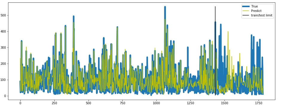
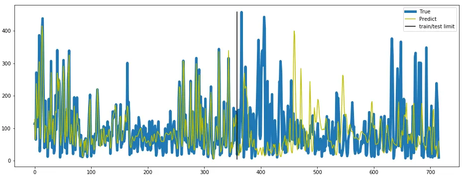
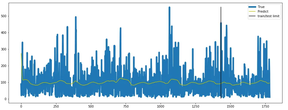
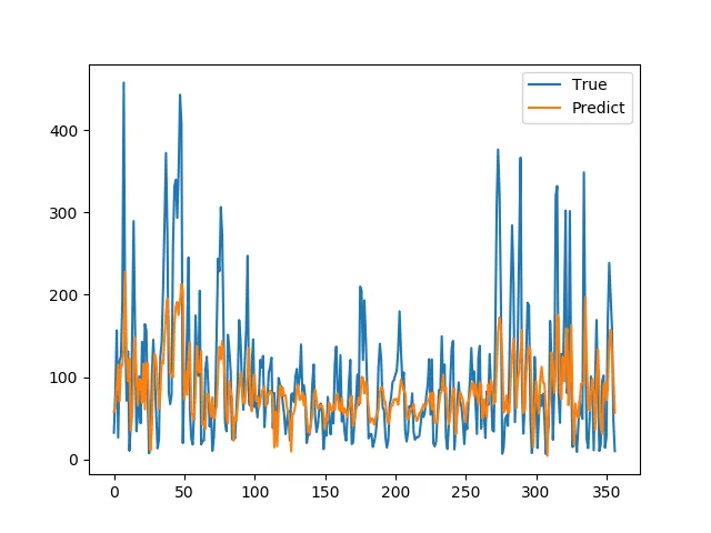
plt.plot(y_test, label='True')
plt.plot(y_predict, label='Predict')
plt.legend()
plt.show()
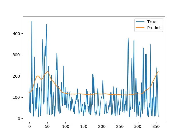
但预测非常差。如何改进预测?您有任何改进的想法吗?
通过重新设计架构和/或层,有没有改进预测的想法?