如果我想对随机非结构化数据进行3D样条/平滑插值，应该怎么做？

Question

如果我想对随机非结构化数据进行3D样条/平滑插值，应该怎么做？

21

我受到@James的这个答案的启发，想看看如何使用griddata和map_coordinates。在下面的例子中，我展示了2D数据，但我的兴趣在于3D。我注意到griddata仅为1D和2D提供样条插值，并且仅限于线性插值用于3D及更高维度（可能是出于非常好的原因）。然而，map_coordinates似乎可以使用高阶（比分段线性更平滑）插值来处理3D。

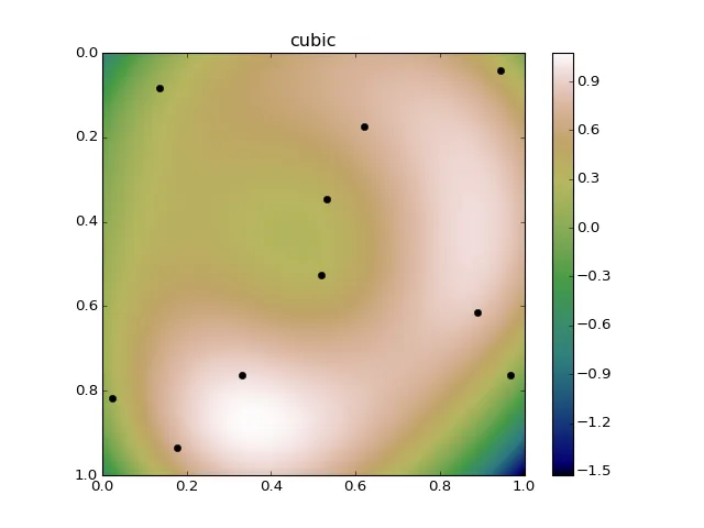
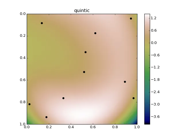
我的主要问题：如果我有随机的非结构化数据（无法使用map_coordinates），在NumPy SciPy宇宙中是否有某种方法可以获得比分段线性插值更平滑的插值，或者至少附近？

我的次要问题：3D的样条插值在griddata中不可用，是因为实现困难或繁琐，还是存在根本性的困难？

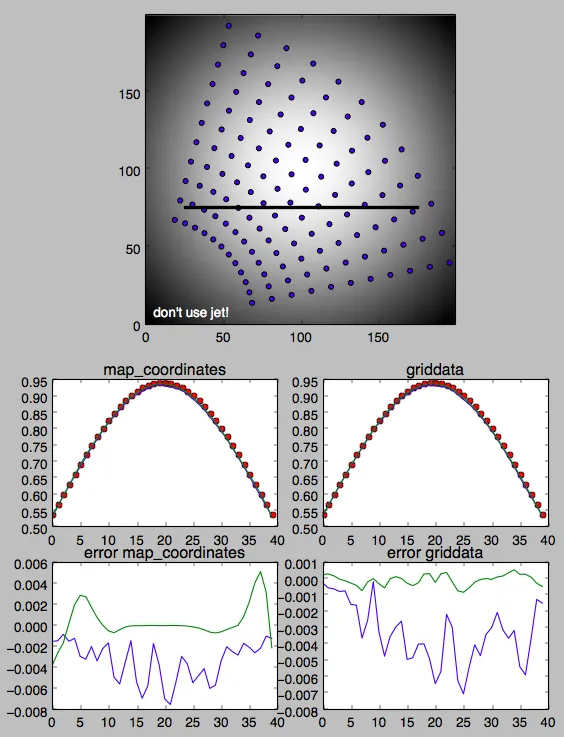
下面的图片和可怕的Python代码展示了我对griddata和map_coordinates的理解。插值沿着粗黑线进行。

结构化数据：

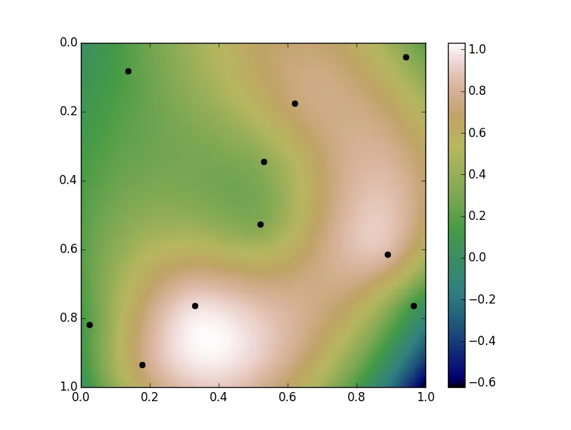
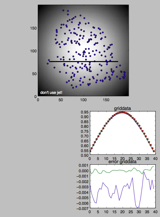
非结构化数据：

可怕的 Python：

import numpy as np
import matplotlib.pyplot as plt

def g(x, y):
    return np.exp(-((x-1.0)**2 + (y-1.0)**2))

def findit(x, X):  # or could use some 1D interpolation
    fraction = (x - X[0]) / (X[-1]-X[0])
    return fraction * float(X.shape[0]-1)

nth, nr = 12, 11
theta_min, theta_max = 0.2, 1.3
r_min,     r_max     = 0.7, 2.0

theta = np.linspace(theta_min, theta_max, nth)
r     = np.linspace(r_min,     r_max,     nr)

R, TH = np.meshgrid(r, theta)
Xp, Yp  = R*np.cos(TH), R*np.sin(TH)
array = g(Xp, Yp)

x, y = np.linspace(0.0, 2.0, 200), np.linspace(0.0, 2.0, 200)
X, Y = np.meshgrid(x, y)
blob = g(X, Y)

xtest = np.linspace(0.25, 1.75, 40)
ytest = np.zeros_like(xtest) + 0.75

rtest = np.sqrt(xtest**2 + ytest**2)
thetatest = np.arctan2(xtest, ytest)

ir = findit(rtest, r)
it = findit(thetatest, theta)

plt.figure()

plt.subplot(2,1,1)

plt.scatter(100.0*Xp.flatten(), 100.0*Yp.flatten())
plt.plot(100.0*xtest, 100.0*ytest, '-k', linewidth=3)
plt.hold
plt.imshow(blob, origin='lower', cmap='gray')

plt.text(5, 5, "don't use jet!", color='white')


exact = g(xtest, ytest)

import scipy.ndimage.interpolation as spndint
ndint0 = spndint.map_coordinates(array, [it, ir], order=0)
ndint1 = spndint.map_coordinates(array, [it, ir], order=1)
ndint2 = spndint.map_coordinates(array, [it, ir], order=2)

import scipy.interpolate as spint
points = np.vstack((Xp.flatten(), Yp.flatten())).T   # could use np.array(zip(...))
grid_x = xtest
grid_y = np.array([0.75])

g0 = spint.griddata(points, array.flatten(), (grid_x, grid_y), method='nearest')
g1 = spint.griddata(points, array.flatten(), (grid_x, grid_y), method='linear')
g2 = spint.griddata(points, array.flatten(), (grid_x, grid_y), method='cubic')


plt.subplot(4,2,5)

plt.plot(exact, 'or')
#plt.plot(ndint0)
plt.plot(ndint1)
plt.plot(ndint2)
plt.title("map_coordinates")

plt.subplot(4,2,6)

plt.plot(exact, 'or')
#plt.plot(g0)
plt.plot(g1)
plt.plot(g2)
plt.title("griddata")

plt.subplot(4,2,7)

#plt.plot(ndint0 - exact)
plt.plot(ndint1 - exact)
plt.plot(ndint2 - exact)
plt.title("error map_coordinates")

plt.subplot(4,2,8)

#plt.plot(g0 - exact)
plt.plot(g1 - exact)
plt.plot(g2 - exact)
plt.title("error griddata")

plt.show()


seed_points_rand = 2.0 * np.random.random((400, 2))
rr = np.sqrt((seed_points_rand**2).sum(axis=-1))
thth = np.arctan2(seed_points_rand[...,1], seed_points_rand[...,0])
isinside = (rr>r_min) * (rr<r_max) * (thth>theta_min) * (thth<theta_max)
points_rand = seed_points_rand[isinside]

Xprand, Yprand = points_rand.T  # unpack
array_rand = g(Xprand, Yprand)

grid_x = xtest
grid_y = np.array([0.75])

plt.figure()

plt.subplot(2,1,1)

plt.scatter(100.0*Xprand.flatten(), 100.0*Yprand.flatten())
plt.plot(100.0*xtest, 100.0*ytest, '-k', linewidth=3)
plt.hold
plt.imshow(blob, origin='lower', cmap='gray')
plt.text(5, 5, "don't use jet!", color='white')


g0rand = spint.griddata(points_rand, array_rand.flatten(), (grid_x, grid_y), method='nearest')
g1rand = spint.griddata(points_rand, array_rand.flatten(), (grid_x, grid_y), method='linear')
g2rand = spint.griddata(points_rand, array_rand.flatten(), (grid_x, grid_y), method='cubic')

plt.subplot(4,2,6)

plt.plot(exact, 'or')
#plt.plot(g0rand)
plt.plot(g1rand)
plt.plot(g2rand)
plt.title("griddata")


plt.subplot(4,2,8)

#plt.plot(g0rand - exact)
plt.plot(g1rand - exact)
plt.plot(g2rand - exact)
plt.title("error griddata")

plt.show()

- uhoh

1个回答

网页内容由stack overflow 提供, 点击上面的

可以查看英文原文，
原文链接

- Joe Kington · Accepted Answer

好问题！（还有漂亮的图表！）

对于非结构化数据，您需要切换回针对非结构化数据的函数。 griddata 是一种选择，但会在三角形边界处使用三角剖分和线性插值，从而导致“硬”边缘。

Splines 是径向基函数。按照 scipy 的术语，您需要使用 scipy.interpolate.Rbf。我建议使用 function="linear" 或 function="thin_plate" 而不是三次样条，但也可以使用三次样条。（与线性或薄板样条相比，三次样条将加剧“过冲”问题。）

一个注意点是，径向基函数的这个特定实现将始终使用数据集中的所有点。这是最准确和平滑的方法，但随着输入观测点数量的增加，它的可扩展性较差。有几种解决方法，但问题会变得更加复杂。我将把它留给另一个问题。

无论如何，这里是一个简化的示例。我们将生成随机数据，然后在位于正则网格上的点上进行插值。（请注意，输入不在规则网格上，并且插值点也不需要是规则的。）

import numpy as np
import scipy.interpolate
import matplotlib.pyplot as plt
np.random.seed(1977)

x, y, z = np.random.random((3, 10))

interp = scipy.interpolate.Rbf(x, y, z, function='thin_plate')

yi, xi = np.mgrid[0:1:100j, 0:1:100j]

zi = interp(xi, yi)

plt.plot(x, y, 'ko')
plt.imshow(zi, extent=[0, 1, 1, 0], cmap='gist_earth')
plt.colorbar()

plt.show()

样条函数的选择

我选择了"thin_plate"作为样条函数的类型。我们的输入观测点范围从0到1（它们是由 np.random.random 创建的）。请注意，我们的插值值略高于1，远低于零。这就是"过冲"。

线性样条将完全避免出现过冲，但您最终会得到“靶心”图案（虽然与IDW方法相比不会那么严重）。例如，以下是使用线性径向基函数插值的完全相同数据。请注意，我们的插值值永远不会超过1或低于0：

更高阶的样条函数将使数据中的趋势更连续，但会产生更多的过冲。默认的"multiquadric"与薄板样条函数非常相似，但会使事物更连续并且过冲更严重：

然而，当你使用更高阶的样条函数时，比如"cubic"(三阶)：

和"quintic"(五阶)

你会发现即使稍微超出输入数据，也可能得到不合理的结果。

无论如何，以下是一个简单的示例，用于比较随机数据上的不同径向基函数:

import numpy as np
import scipy.interpolate
import matplotlib.pyplot as plt
np.random.seed(1977)

x, y, z = np.random.random((3, 10))
yi, xi = np.mgrid[0:1:100j, 0:1:100j]

interp_types = ['multiquadric', 'inverse', 'gaussian', 'linear', 'cubic',
                'quintic', 'thin_plate']

for kind in interp_types:
    interp = scipy.interpolate.Rbf(x, y, z, function=kind)
    zi = interp(xi, yi)

    fig, ax = plt.subplots()
    ax.plot(x, y, 'ko')
    im = ax.imshow(zi, extent=[0, 1, 1, 0], cmap='gist_earth')
    fig.colorbar(im)
    ax.set(title=kind)
    fig.savefig(kind + '.png', dpi=80)

plt.show()