为什么我的卷积例程与NumPy和SciPy的不同？

Question

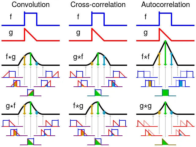
我想手动编写一个一维卷积，因为我正在尝试使用核对时间序列进行分类，并决定制作著名的维基百科卷积图像，如此处所示。

这是我的脚本。我正在使用数字信号卷积的标准公式。

import numpy as np 
import matplotlib.pyplot as plt
import scipy.ndimage

plt.style.use('ggplot')

def convolve1d(signal, ir):
    """
    we use the 'same' / 'constant' method for zero padding. 
    """
    n = len(signal)
    m = len(ir)
    output = np.zeros(n)

    for i in range(n):
        for j in range(m):
            if i - j < 0: continue
            output[i] += signal[i - j] * ir[j]

    return output

def make_square_and_saw_waves(height, start, end, n):
    single_square_wave = []
    single_saw_wave = []
    for i in range(n):
        if start <= i < end:
            single_square_wave.append(height)
            single_saw_wave.append(height * (end-i) / (end-start))
        else:
            single_square_wave.append(0)
            single_saw_wave.append(0)

    return single_square_wave, single_saw_wave

# create signal and IR
start = 40
end = 60
single_square_wave, single_saw_wave = make_square_and_saw_waves(
    height=10, start=start, end=end, n=100)

# convolve, compare different methods
np_conv = np.convolve(
    single_square_wave, single_saw_wave, mode='same')

convolution1d = convolve1d(
    single_square_wave, single_saw_wave)

sconv = scipy.ndimage.convolve1d(
    single_square_wave, single_saw_wave, mode='constant')

# plot them, scaling by the height
plt.clf()
fig, axs = plt.subplots(5, 1, figsize=(12, 6), sharey=True, sharex=True)

axs[0].plot(single_square_wave / np.max(single_square_wave), c='r')
axs[0].set_title('Single Square')
axs[0].set_ylim(-.1, 1.1)

axs[1].plot(single_saw_wave / np.max(single_saw_wave), c='b')
axs[1].set_title('Single Saw')
axs[2].set_ylim(-.1, 1.1)

axs[2].plot(convolution1d / np.max(convolution1d), c='g')
axs[2].set_title('Our Convolution')
axs[2].set_ylim(-.1, 1.1)

axs[3].plot(np_conv / np.max(np_conv), c='g')
axs[3].set_title('Numpy Convolution')
axs[3].set_ylim(-.1, 1.1)

axs[4].plot(sconv / np.max(sconv), c='purple')
axs[4].set_title('Scipy Convolution')
axs[4].set_ylim(-.1, 1.1)

plt.show()

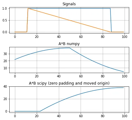
以下是我得到的情节：

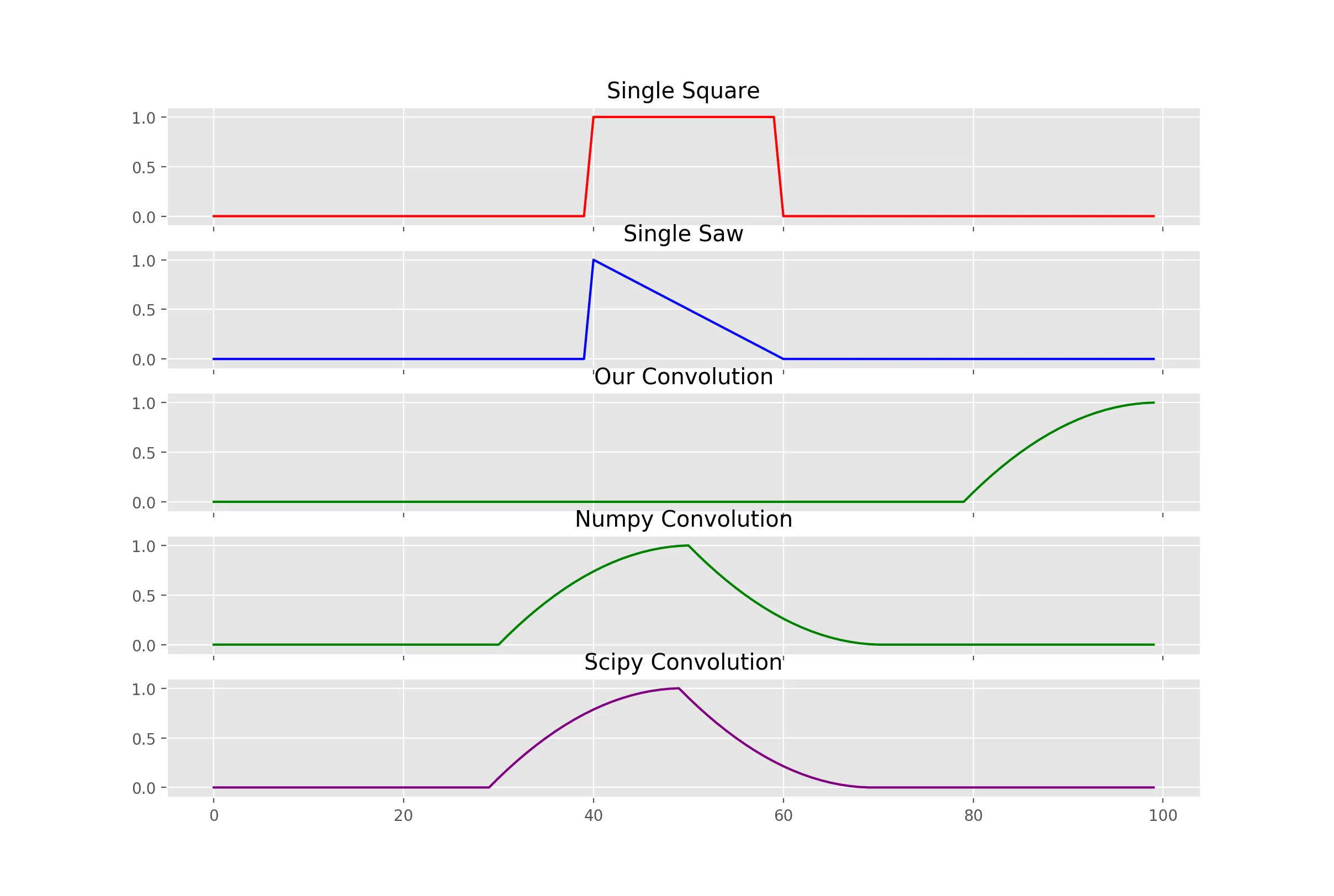
正如您所看到的，由于某种原因，我的卷积被移位了。曲线中的数字（y值）是相同的，但是移位了约一半的滤波器大小。

有人知道这是怎么回事吗？

- lollercoaster

Answer 1

就像你链接的公式一样，卷积对从负无穷到正无穷的指数求和。对于有限序列，你必须处理不可避免的边界效应。Numpy和scipy提供了不同的处理方式：

numpy convolve：

mode : {‘full’, ‘valid’, ‘same’}, 可选项

scipy convolve：

mode : {‘reflect’,’constant’,’nearest’,’mirror’, ‘wrap’}, 可选项

下一个问题是确定原点位置。在你提供的实现中，你的信号从 t=0 开始，并且舍弃了负 t 的所有项。Scipy 提供了一个参数 origin 来考虑这个问题。

origin : array_like, 可选项 origin 参数用于控制过滤器的放置。默认值为 0。

你可以使用 scipy 的 convolve 来模仿你的实现行为：

from scipy.ndimage.filters import convolve as convolve_sci
from pylab import *

N = 100
start=N//8
end = N-start
A = zeros(N)
A[start:end] = 1
B = zeros(N)
B[start:end] = linspace(1,0,end-start)

figure(figsize=(6,7))
subplot(411); grid(); title('Signals')
plot(A)
plot(B)
subplot(412); grid(); title('A*B numpy')
plot(convolve(A,B, mode='same'))
subplot(413); grid(); title('A*B scipy (zero padding and moved origin)')
plot(convolve_sci(A,B, mode='constant', origin=-N//2))
tight_layout()
show()

简言之，在进行卷积操作时，您需要决定如何处理序列之外的数值（例如将其设置为零（numpy），反射，包装等），以及信号起点的位置。

请注意，numpy和scipy的默认设置在如何处理边缘效应方面也存在差异（零填充vs反射）。

- Jul3k

Answer 2

首先，为了符合文档的表示法，output[i] += signal[i - j] * ir[j] 应该改为 output[i] += signal[j] * ir[i - j] 使用文档中的变量名称可以使其更加易懂：

i = len(signal)
for n in range(i):
    for k in range(n):
        output[n] += signal[k] * ir[n - k]

您能够成功实现这一点是因为卷积运算满足交换律，所以 f*g == g*f（请参见您的图表）。

然而，主要区别在于长度为 m 的信号和长度为 n 的脉冲的“基本”卷积结果长度为 m + n -1（请参见 np.convolve 文档），但是 np.convolve( . . . , mode = 'same') 和 scipy.ndimage.convolve1d 都通过从信号两端裁剪元素来返回长度为 m 的信号。

因此，您的问题在于您只从右侧裁剪了信号，这就是为什么……

np.all(
       np.convolve(single_square_wave, single_saw_wave)[:len(single_square_wave)]\
       ==\
       convolve1d(single_square_wave, single_saw_wave)
       )

True

为了做与np.convolve(..., mode = 'same')相同的修剪，你需要：

def convolve1d_(signal, ir):
    """
    we use the 'same' / 'constant' method for zero padding. 
    """
    pad = len(ir)//2 - 1
    n_ = range(pad, pad + len(signal))
    output = np.zeros(pad + len(signal))

    for n in n_:
        kmin = max(0, n - len(ir) + 1)
        kmax = min(len(ir), n)
        for k in range(kmin, kmax):
            output[n] += signal[k] * ir[n - k]

    return output[pad:]

测试：

np.all(
       np.convolve(single_square_wave, single_saw_wave, mode = 'same')\
       ==\
       convolve1d_(single_square_wave,single_saw_wave)
       )

True

- Daniel F

---

你的代码不再正确，例如：np.convolve([1,2,3],[0,1,0.5],'same')和convolve1d_([1,2,3],[0,1,0.5])的结果不同。我对Numpy的文档感到困惑，仍然无法理解“same”是如何实现的。 - SiXUlm