给定两个函数,我想找出它们的公共切线:
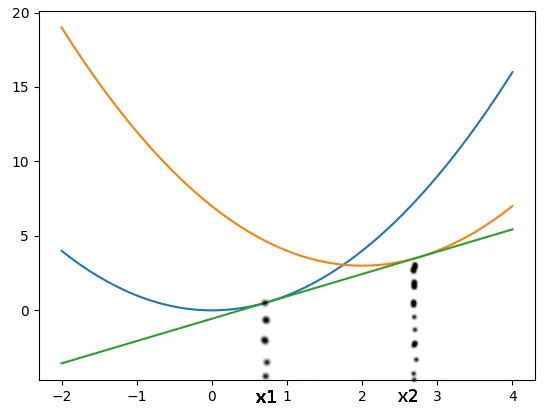
公共切线的斜率可以通过以下方式获得:
slope of common tangent = (f(x1) - g(x2)) / (x1 - x2) = f'(x1) = g'(x2)
因此,最终我们将得到一个包含两个未知数的2元方程组:
f'(x1) = g'(x2) # Eq. 1
(f(x1) - g(x2)) / (x1 - x2) = f'(x1) # Eq. 2
由于某些我不理解的原因,Python未找到解决方案:
import numpy as np
from scipy.optimize import curve_fit
import matplotlib.pyplot as plt
import sys
from sympy import *
import sympy as sym


# Intial candidates for fit
E0_init = -941.510817926696
V0_init = 63.54960592453
B0_init = 76.3746233515232
B0_prime_init = 4.05340727164527

# Data 1 (Red triangles):
V_C_I, E_C_I = np.loadtxt('./1.dat', skiprows = 1).T

# Data 14 (Empty grey triangles):
V_14, E_14 = np.loadtxt('./2.dat', skiprows = 1).T

def BM(x, a, b, c, d):
        return  (2.293710449E+17)*(1E-21)* (a + b*x + c*x**2 + d*x**3 )

def P(x, b, c, d):
    return -b - 2*c*x - 3 *d*x**2

init_vals = [E0_init, V0_init, B0_init, B0_prime_init]
popt_C_I, pcov_C_I = curve_fit(BM, V_C_I, E_C_I, p0=init_vals)
popt_14, pcov_14 = curve_fit(BM, V_14, E_14, p0=init_vals)

x1 = var('x1')
x2 = var('x2')

E1 = P(x1, popt_C_I[1], popt_C_I[2], popt_C_I[3]) - P(x2, popt_14[1], popt_14[2], popt_14[3])
print 'E1 = ', E1

E2 = ((BM(x1, popt_C_I[0], popt_C_I[1], popt_C_I[2], popt_C_I[3]) - BM(x2, popt_14[0], popt_14[1], popt_14[2], popt_14[3])) / (x1 - x2)) - P(x1, popt_C_I[1], popt_C_I[2], popt_C_I[3])

sols = solve([E1, E2], [x1, x2])

print 'sols = ', sols

# Linspace for plotting the fitting curves:
V_C_I_lin = np.linspace(V_C_I[0], V_C_I[-1], 10000)
V_14_lin = np.linspace(V_14[0], V_14[-1], 10000)

plt.figure()
# Plotting the fitting curves:
p2, = plt.plot(V_C_I_lin, BM(V_C_I_lin, *popt_C_I), color='black', label='Cubic fit data 1' )
p6, = plt.plot(V_14_lin, BM(V_14_lin, *popt_14), 'b', label='Cubic fit data 2')

# Plotting the scattered points:
p1 = plt.scatter(V_C_I, E_C_I, color='red', marker="^", label='Data 1', s=100)
p5 = plt.scatter(V_14, E_14, color='grey', marker="^", facecolors='none', label='Data 2', s=100)

plt.ticklabel_format(useOffset=False)
plt.show()
1.dat 的内容如下:
61.6634100000000 -941.2375622594436
62.3429030000000 -941.2377748739724
62.9226515000000 -941.2378903605746
63.0043440000000 -941.2378981684135
63.7160150000000 -941.2378864590100
64.4085050000000 -941.2377753645115
65.1046835000000 -941.2375332100225
65.8049585000000 -941.2372030376584
66.5093925000000 -941.2367456992965
67.2180970000000 -941.2361992239395
67.9311515000000 -941.2355493856510
2.dat 是以下内容:
54.6569312500000 -941.2300821583739
55.3555152500000 -941.2312112888004
56.1392347500000 -941.2326135552780
56.9291575000000 -941.2338291772218
57.6992532500000 -941.2348135408652
58.4711572500000 -941.2356230099117
59.2666985000000 -941.2362715934311
60.0547935000000 -941.2367074271724
60.8626545000000 -941.2370273047416
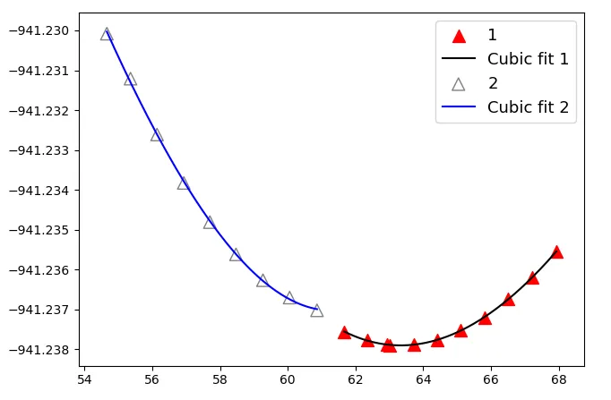
更新:使用@if...方法:
import numpy as np
from scipy.optimize import curve_fit
import matplotlib.pyplot as plt
from matplotlib.font_manager import FontProperties

# Intial candidates for fit, per FU: - thus, the E vs V input data has to be per FU
E0_init = -941.510817926696
V0_init = 63.54960592453
B0_init = 76.3746233515232
B0_prime_init = 4.05340727164527

def BM(x, a, b, c, d):
         return  a + b*x + c*x**2 + d*x**3

def devBM(x, b, c, d):
         return  b + 2*c*x + 3*d*x**2

# Data 1 (Red triangles):
V_C_I, E_C_I = np.loadtxt('./1.dat', skiprows = 1).T

# Data 14 (Empty grey triangles):
V_14, E_14 = np.loadtxt('./2.dat', skiprows = 1).T

init_vals = [E0_init, V0_init, B0_init, B0_prime_init]
popt_C_I, pcov_C_I = curve_fit(BM, V_C_I, E_C_I, p0=init_vals)
popt_14, pcov_14 = curve_fit(BM, V_14, E_14, p0=init_vals)

from scipy.optimize import fsolve
def equations(p):
    x1, x2 = p
    E1 = devBM(x1, popt_C_I[1], popt_C_I[2], popt_C_I[3]) - devBM(x2, popt_14[1], popt_14[2], popt_14[3])
    E2 = ((BM(x1, popt_C_I[0], popt_C_I[1], popt_C_I[2], popt_C_I[3]) - BM(x2, popt_14[0], popt_14[1], popt_14[2], popt_14[3])) / (x1 - x2)) - devBM(x1, popt_C_I[1], popt_C_I[2], popt_C_I[3])
    return (E1, E2)

x1, x2 =  fsolve(equations, (50, 60))
print 'x1 = ', x1
print 'x2 = ', x2

slope_common_tangent = devBM(x1, popt_C_I[1], popt_C_I[2], popt_C_I[3])
print 'slope_common_tangent = ', slope_common_tangent

def comm_tangent(x, x1, slope_common_tangent):
   return BM(x1, popt_C_I[0], popt_C_I[1], popt_C_I[2], popt_C_I[3]) - slope_common_tangent * x1 + slope_common_tangent * x

# Linspace for plotting the fitting curves:
V_C_I_lin = np.linspace(V_C_I[0], V_C_I[-1], 10000)
V_14_lin = np.linspace(V_14[0], V_14[-1], 10000)

plt.figure()

# Plotting the fitting curves:
p2, = plt.plot(V_C_I_lin, BM(V_C_I_lin, *popt_C_I), color='black', label='Cubic fit Calcite I' )
p6, = plt.plot(V_14_lin, BM(V_14_lin, *popt_14), 'b', label='Cubic fit Calcite II')

xp = np.linspace(54, 68, 100)
pcomm_tangent, = plt.plot(xp, comm_tangent(xp, x1, slope_common_tangent), 'green', label='Common tangent')

# Plotting the scattered points:
p1 = plt.scatter(V_C_I, E_C_I, color='red', marker="^", label='Calcite I', s=100)
p5 = plt.scatter(V_14, E_14, color='grey', marker="^", facecolors='none', label='Calcite II', s=100)

fontP = FontProperties()
fontP.set_size('13')

plt.legend((p1, p2, p5, p6, pcomm_tangent), ("1", "Cubic fit 1", "2", 'Cubic fit 2', 'Common tangent'), prop=fontP)

print 'devBM(x1, popt_C_I[1], popt_C_I[2], popt_C_I[3]) = ', devBM(x1, popt_C_I[1], popt_C_I[2], popt_C_I[3])

plt.ylim(-941.240, -941.225)
plt.ticklabel_format(useOffset=False)

plt.show()
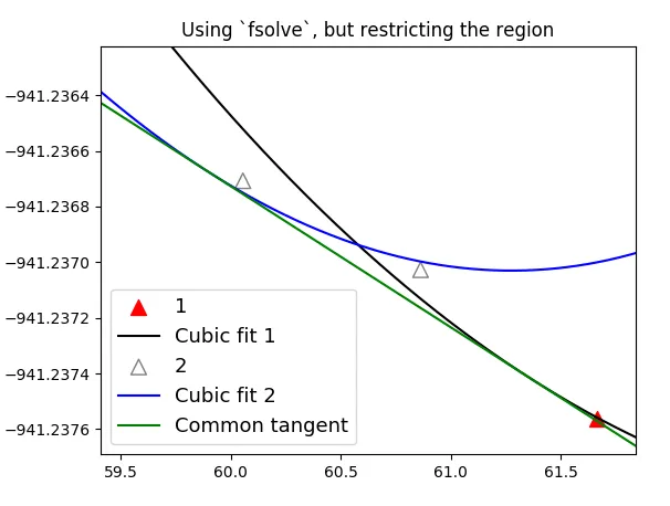
我能找到共切线,如下所示:
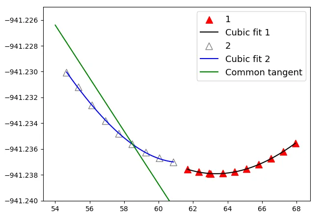
然而,这个共切线对应于数据范围之外的区域,即使用
V_C_I_lin = np.linspace(V_C_I[0]-30, V_C_I[-1], 10000)
V_14_lin = np.linspace(V_14[0]-20, V_14[-1]+2, 10000)
xp = np.linspace(40, 70, 100)
plt.ylim(-941.25, -941.18)
可以看到以下内容:
是否可以将求解器限制在数据范围内,以便找到所需的公切线?
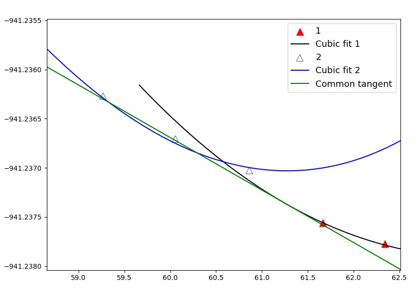
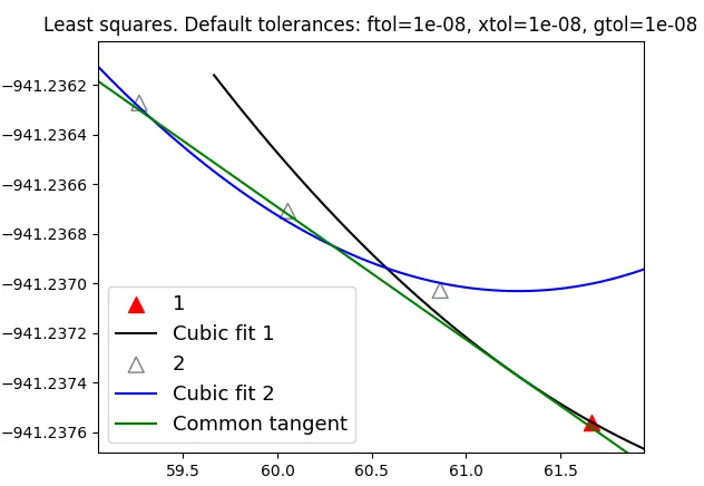
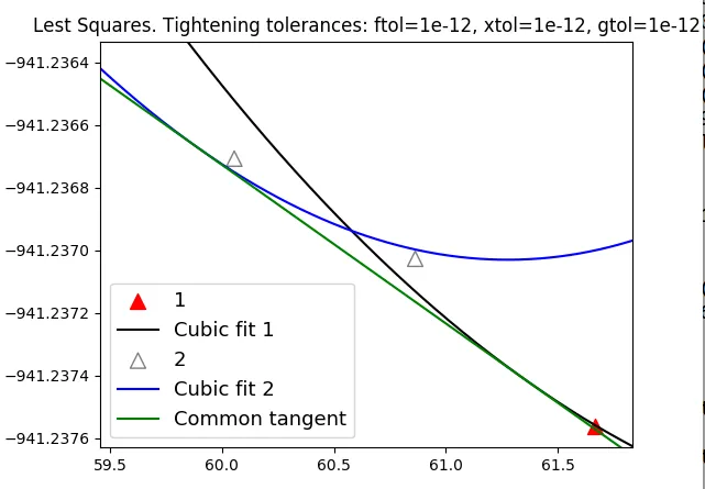
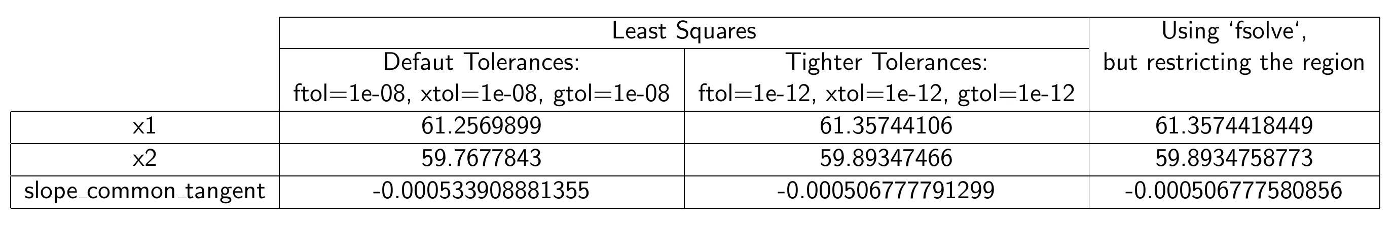
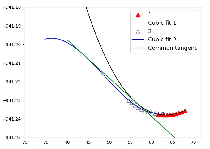
更新2.1:使用@if...范围约束方法,以下代码产生x1=61.2569899和x2=59.7677843。如果我们绘制它:
import numpy as np
from scipy.optimize import curve_fit
import matplotlib.pyplot as plt
from matplotlib.font_manager import FontProperties
import sys
from sympy import *
import sympy as sym
import os

# Intial candidates for fit, per FU: - thus, the E vs V input data has to be per FU
E0_init = -941.510817926696  # -1882.50963222/2.0
V0_init = 63.54960592453 #125.8532/2.0
B0_init = 76.3746233515232 #74.49
B0_prime_init = 4.05340727164527 #4.15

def BM(x, a, b, c, d):
         return  a + b*x + c*x**2 + d*x**3

def devBM(x, b, c, d):
         return  b + 2*c*x + 3*d*x**2

# Data 1 (Red triangles):
V_C_I, E_C_I = np.loadtxt('./1.dat', skiprows = 1).T

# Data 14 (Empty grey triangles):
V_14, E_14 = np.loadtxt('./2.dat', skiprows = 1).T

init_vals = [E0_init, V0_init, B0_init, B0_prime_init]
popt_C_I, pcov_C_I = curve_fit(BM, V_C_I, E_C_I, p0=init_vals)
popt_14, pcov_14 = curve_fit(BM, V_14, E_14, p0=init_vals)

def equations(p):
    x1, x2 = p
    E1 = devBM(x1, popt_C_I[1], popt_C_I[2], popt_C_I[3]) - devBM(x2, popt_14[1], popt_14[2], popt_14[3])
    E2 = ((BM(x1, popt_C_I[0], popt_C_I[1], popt_C_I[2], popt_C_I[3]) - BM(x2, popt_14[0], popt_14[1], popt_14[2], popt_14[3])) / (x1 - x2)) - devBM(x1, popt_C_I[1], popt_C_I[2], popt_C_I[3])
    return (E1, E2)

from scipy.optimize import least_squares
lb = (61.0, 59.0)   # lower bounds on x1, x2
ub = (62.0, 60.0)    # upper bounds
result = least_squares(equations, [61, 59], bounds=(lb, ub))
print 'result = ', result

# The result obtained is:
# x1 = 61.2569899
# x2 = 59.7677843

slope_common_tangent = devBM(x1, popt_C_I[1], popt_C_I[2], popt_C_I[3])
print 'slope_common_tangent = ', slope_common_tangent


def comm_tangent(x, x1, slope_common_tangent):
   return BM(x1, popt_C_I[0], popt_C_I[1], popt_C_I[2], popt_C_I[3]) - slope_common_tangent * x1 + slope_common_tangent * x

# Linspace for plotting the fitting curves:
V_C_I_lin = np.linspace(V_C_I[0]-2, V_C_I[-1], 10000)
V_14_lin = np.linspace(V_14[0], V_14[-1]+2, 10000)


fig_handle = plt.figure()

# Plotting the fitting curves:
p2, = plt.plot(V_C_I_lin, BM(V_C_I_lin, *popt_C_I), color='black' )
p6, = plt.plot(V_14_lin, BM(V_14_lin, *popt_14), 'b' )

xp = np.linspace(54, 68, 100)
pcomm_tangent, = plt.plot(xp, comm_tangent(xp, x1, slope_common_tangent), 'green', label='Common tangent')

# Plotting the scattered points:
p1 = plt.scatter(V_C_I, E_C_I, color='red', marker="^", label='1', s=100)
p5 = plt.scatter(V_14, E_14, color='grey', marker="^", facecolors='none', label='2', s=100)

fontP = FontProperties()
fontP.set_size('13')

plt.legend((p1, p2, p5, p6, pcomm_tangent), ("1", "Cubic fit 1", "2", 'Cubic fit 2', 'Common tangent'), prop=fontP)


plt.ticklabel_format(useOffset=False)

plt.show()
我们发现我们没有得到公共切线: