我将借用以下stackoverflow问题的图片来描述我的问题:
Drawing decision boundary of two multivariate gaussian
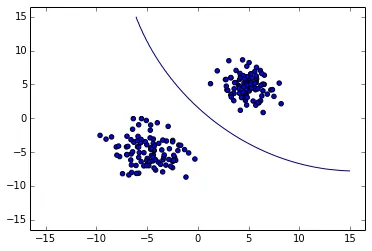
我有2个带有2D点的类,我感兴趣的是决策边界(或判别式)。
我编写了返回判别函数结果(浮点值)的函数,这使我能够将样本分类为这两种模式。
如果一个样本点是例如,x_i = [x, y] 我可以调用函数
如果g1(x,y) > g2(x,y),它属于类1,反之亦然,如果g1(x,y) <= g2(x,y),它属于类2
因此,决策边界应该在g1(x,y) == g2(x,y)处。
编辑:
希望示例有所帮助:
1) 假设我从数据集中取1个样本x=[1,2]
2) 然后我会调用例如: g1(1,2) --> 返回0.345 g2(1,2) --> 返回0.453 --> 样本x属于类2,因为g2(1,2)>g1(1,2)
3) 现在对于决策边界,我有g2(x,y)==g1(x,y),或者g1(x,y)-g2(x,y)==0
4) 我生成一系列x值,例如1,2,3,4,5,并且现在我想找到对应的y值,使得g1(x,y)-g2(x,y)==0
5) 然后我可以使用这些x,y对来绘制决策边界。
在我上面链接的StackOverflow帖子中,建议是:
您可以简单地绘制f(x,y)的等高线:= pdf1(x,y)>pdf2(x,y)。因此,您定义函数f为1,当且仅当pdf1(x,y)> pdf2(x,y)时。这样,唯一的等高线将沿着pdf1(x,y)== pdf2(x,y)的曲线放置,这是决策边界(判别式)。如果您希望定义“好”的函数,只需设置f(x,y)= sgn(pdf1(x,y)- pdf2(x,y)),并绘制其等高线图将得到完全相同的判别式。
当我执行它时,它将返回一个浮点数,例如,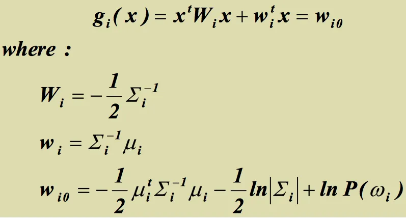 非常感谢对等高线的建议,但是我在实现中遇到了问题:
我编写了返回判别函数结果(浮点值)的函数,这使我能够将样本分类为这两种模式。
如果一个样本点是例如,x_i = [x, y] 我可以调用函数
如果g1(x,y) > g2(x,y),它属于类1,反之亦然,如果g1(x,y) <= g2(x,y),它属于类2
因此,决策边界应该在g1(x,y) == g2(x,y)处。
编辑:
希望示例有所帮助:
1) 假设我从数据集中取1个样本x=[1,2]
2) 然后我会调用例如: g1(1,2) --> 返回0.345 g2(1,2) --> 返回0.453 --> 样本x属于类2,因为g2(1,2)>g1(1,2)
3) 现在对于决策边界,我有g2(x,y)==g1(x,y),或者g1(x,y)-g2(x,y)==0
4) 我生成一系列x值,例如1,2,3,4,5,并且现在我想找到对应的y值,使得g1(x,y)-g2(x,y)==0
5) 然后我可以使用这些x,y对来绘制决策边界。
在我上面链接的StackOverflow帖子中,建议是:
您可以简单地绘制f(x,y)的等高线:= pdf1(x,y)>pdf2(x,y)。因此,您定义函数f为1,当且仅当pdf1(x,y)> pdf2(x,y)时。这样,唯一的等高线将沿着pdf1(x,y)== pdf2(x,y)的曲线放置,这是决策边界(判别式)。如果您希望定义“好”的函数,只需设置f(x,y)= sgn(pdf1(x,y)- pdf2(x,y)),并绘制其等高线图将得到完全相同的判别式。
但我该如何在Python和matplotlib中实现它?我真的很迷失,无法设置代码来完成这个任务。感谢您的任何帮助!
编辑:
关于函数g()本身的更多信息:
def discr_func(x, y, cov_mat, mu_vec):
    """
    Calculates the value of the discriminant function for a dx1 dimensional
    sample given covariance matrix and mean vector.

    Keyword arguments:
        x_vec: A dx1 dimensional numpy array representing the sample.
        cov_mat: dxd numpy array of the covariance matrix.
        mu_vec: dx1 dimensional numpy array of the sample mean.

    Returns a float value as result of the discriminant function.

    """
    x_vec = np.array([[x],[y]])

    W_i = (-1/2) * np.linalg.inv(cov_mat)
    assert(W_i.shape[0] > 1 and W_i.shape[1] > 1), 'W_i must be a matrix'

    w_i = np.linalg.inv(cov_mat).dot(mu_vec)
    assert(w_i.shape[0] > 1 and w_i.shape[1] == 1), 'w_i must be a column vector'

    omega_i_p1 = (((-1/2) * (mu_vec).T).dot(np.linalg.inv(cov_mat))).dot(mu_vec)
    omega_i_p2 = (-1/2) * np.log(np.linalg.det(cov_mat))
    omega_i = omega_i_p1 - omega_i_p2
    assert(omega_i.shape == (1, 1)), 'omega_i must be a scalar'

    g = ((x_vec.T).dot(W_i)).dot(x_vec) + (w_i.T).dot(x_vec) + omega_i
    return float(g)
当我执行它时,它将返回一个浮点数,例如,
discr_func(1, 2, cov_mat=cov_est_1, mu_vec=mu_est_1)
-3.726426544537969
如果我没有犯错,应该是这个方程:
非常感谢对等高线的建议,但是我在实现中遇到了问题:import pylab as pl
X, Y = np.mgrid[-6:6:100j, -6:6:100j]
x = X.ravel()
y = Y.ravel()
p = (discr_func(x, y, cov_mat=cov_est_1, mu_vec=mu_est_1) -\
discr_func(x, y, cov_mat=cov_est_2, mu_vec=mu_est_2)).reshape(X.shape)
#pl.scatter(X_train[:, 0], X_train[:, 1])
pl.contour(X, Y, p, levels=[0])
---------------------------------------------------------------------------
ValueError Traceback (most recent call last)
<ipython-input-192-28c1c8787237> in <module>()
5 y = Y.ravel()
6
----> 7 p = (discr_func(x, y, cov_mat=cov_est_1, mu_vec=mu_est_1) - discr_func(x, y, cov_mat=cov_est_2, mu_vec=mu_est_2)).reshape(X.shape)
8
9 #pl.scatter(X_train[:, 0], X_train[:, 1])
<ipython-input-184-fd2f8b7fad82> in discr_func(x, y, cov_mat, mu_vec)
25 assert(omega_i.shape == (1, 1)), 'omega_i must be a scalar'
26
---> 27 g = ((x_vec.T).dot(W_i)).dot(x_vec) + (w_i.T).dot(x_vec) + omega_i
28 return float(g)
ValueError: objects are not aligned
我的感觉是传递 .ravel() 列表与我设置的这个函数不兼容... 有什么建议吗?