如何在sklearn的Python中绘制SVM决策边界？

Question

使用sklearn库中的SVM算法，我想绘制数据，并使每个标签用不同的颜色表示。我不想给点着色，而是要填充区域颜色。

现在我的代码如下：

d_pred, d_train_std, d_test_std, l_train, l_test

d_pred是预测标签。 我将绘制d_pred和d_train_std的图形，其形状为：（70000,2），其中X轴是第一列，Y轴是第二列。

谢谢。

- anthonya

---

你到底想绘制什么？你只需要一个散点图还是想要绘制决策面/边界？另外，d_train_std是什么？ - seralouk

谢谢您的回答。我还想绘制决策边界。d_train_std是我已经标准化的训练数据。 - anthonya

请查看我的答案并告诉我。 - seralouk

非常感谢。 - anthonya

我做到了，谢谢。 - anthonya

Answer 1

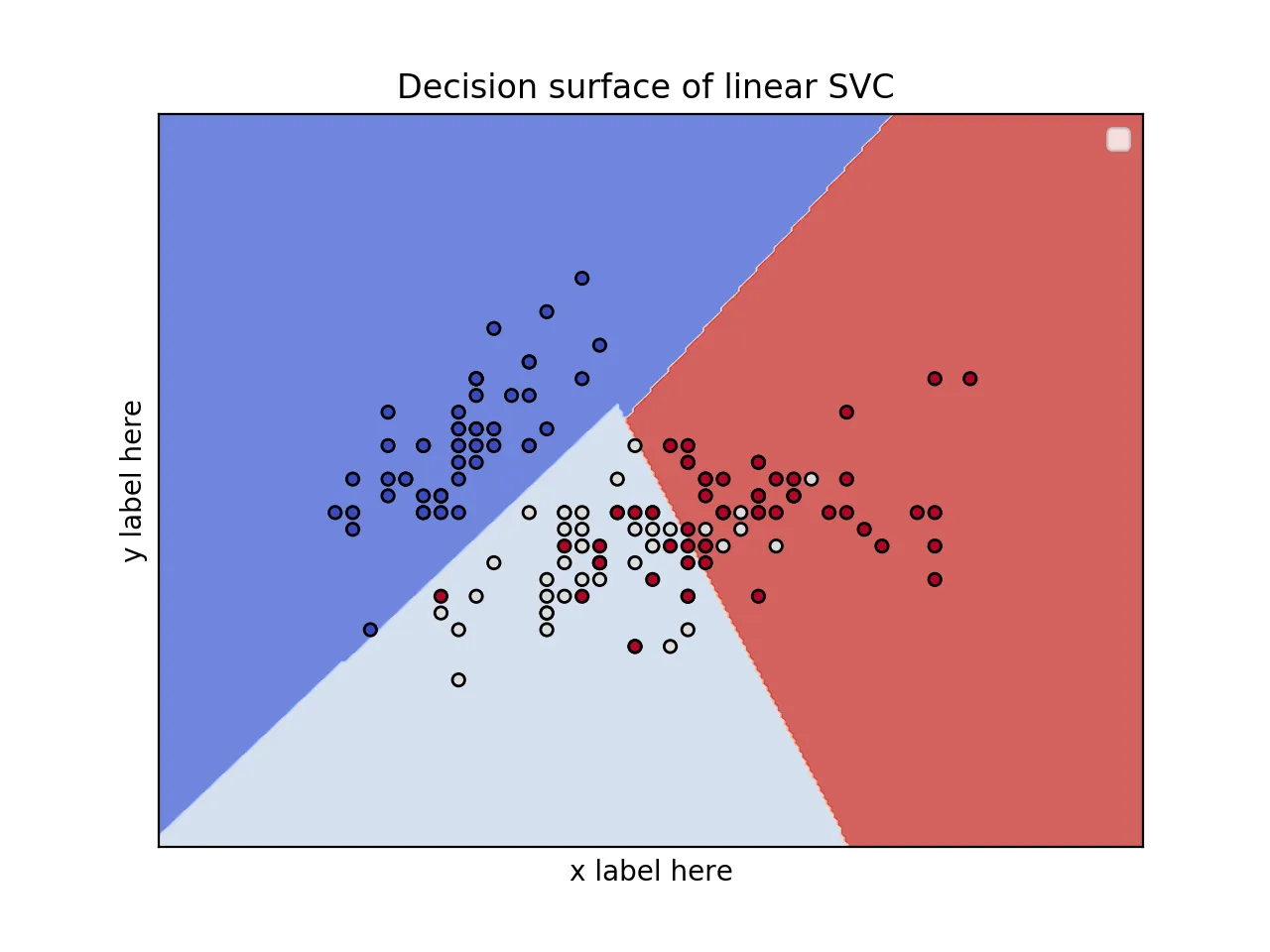
当特征太多时，无法可视化决策面，因为维度太多了，没有办法可视化N维曲面。

然而，你可以使用2个特征并按如下方式绘制出漂亮的决策面。

我还在这里写了一篇文章： https://towardsdatascience.com/support-vector-machines-svm-clearly-explained-a-python-tutorial-for-classification-problems-29c539f3ad8?source=friends_link&sk=80f72ab272550d76a0cc3730d7c8af35

案例1：使用鸢尾花数据集进行2D绘图，并使用2个特征

from sklearn.svm import SVC
import numpy as np
import matplotlib.pyplot as plt
from sklearn import svm, datasets

iris = datasets.load_iris()
X = iris.data[:, :2]  # we only take the first two features.
y = iris.target

def make_meshgrid(x, y, h=.02):
    x_min, x_max = x.min() - 1, x.max() + 1
    y_min, y_max = y.min() - 1, y.max() + 1
    xx, yy = np.meshgrid(np.arange(x_min, x_max, h), np.arange(y_min, y_max, h))
    return xx, yy

def plot_contours(ax, clf, xx, yy, **params):
    Z = clf.predict(np.c_[xx.ravel(), yy.ravel()])
    Z = Z.reshape(xx.shape)
    out = ax.contourf(xx, yy, Z, **params)
    return out

model = svm.SVC(kernel='linear')
clf = model.fit(X, y)

fig, ax = plt.subplots()
# title for the plots
title = ('Decision surface of linear SVC ')
# Set-up grid for plotting.
X0, X1 = X[:, 0], X[:, 1]
xx, yy = make_meshgrid(X0, X1)

plot_contours(ax, clf, xx, yy, cmap=plt.cm.coolwarm, alpha=0.8)
ax.scatter(X0, X1, c=y, cmap=plt.cm.coolwarm, s=20, edgecolors='k')
ax.set_ylabel('y label here')
ax.set_xlabel('x label here')
ax.set_xticks(())
ax.set_yticks(())
ax.set_title(title)
ax.legend()
plt.show()

案例2：使用鸢尾花数据集，绘制三个特征的3D图

from sklearn.svm import SVC
import numpy as np
import matplotlib.pyplot as plt
from sklearn import svm, datasets
from mpl_toolkits.mplot3d import Axes3D

iris = datasets.load_iris()
X = iris.data[:, :3]  # we only take the first three features.
Y = iris.target

#make it binary classification problem
X = X[np.logical_or(Y==0,Y==1)]
Y = Y[np.logical_or(Y==0,Y==1)]

model = svm.SVC(kernel='linear')
clf = model.fit(X, Y)

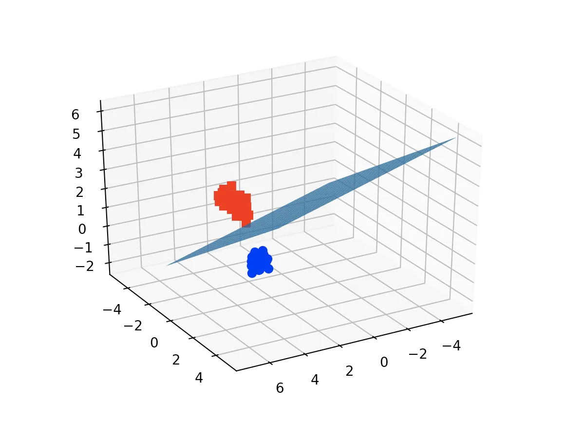
# The equation of the separating plane is given by all x so that np.dot(svc.coef_[0], x) + b = 0.
# Solve for w3 (z)
z = lambda x,y: (-clf.intercept_[0]-clf.coef_[0][0]*x -clf.coef_[0][1]*y) / clf.coef_[0][2]

tmp = np.linspace(-5,5,30)
x,y = np.meshgrid(tmp,tmp)

fig = plt.figure()
ax  = fig.add_subplot(111, projection='3d')
ax.plot3D(X[Y==0,0], X[Y==0,1], X[Y==0,2],'ob')
ax.plot3D(X[Y==1,0], X[Y==1,1], X[Y==1,2],'sr')
ax.plot_surface(x, y, z(x,y))
ax.view_init(30, 60)
plt.show()

- seralouk

Answer 2

这是我的代码，可以实现@Christian Tuchez所描述的功能：

outputs = my_clf.predict(1_test)

hits = []
for i in range(outputs.size):
    if outputs[i] == 1:
        hits.append(i)  # save the index where it's 1

这将保存函数中所有命中点的索引（保存在“hits”列表中）。您可能可以在不使用循环的情况下完成此操作，但我发现这对我来说最容易。

然后要仅显示这些点，您可以编写类似以下内容的代码：

ax.scatter(1_test[hits[:], 0], 1_test[hits[:], 1], 1_test[hits[:], 2], c="cyan", s=2, edgecolor=None)

- Yagoobean

Answer 3

在三维中得到函数可能会很困难。获取可视化的简便方法是获取覆盖您点空间的大量点，并通过您学习的函数（my_model.predict）运行它们，保留击中函数内部的点并对其进行可视化。添加的点越多，边界就越清晰。

- Christian Tuchez

---

这并没有回答问题。一旦您拥有足够的声望，您将能够评论任何帖子；相反，提供不需要询问者澄清的答案。- 来自审核 - Vitalizzare