你需要选择仅两个特征来完成此操作。原因是无法绘制7D图。选择2个特征后,只使用它们来可视化决策面。
(我还在这里写了一篇文章:
https://towardsdatascience.com/support-vector-machines-svm-clearly-explained-a-python-tutorial-for-classification-problems-29c539f3ad8?source=friends_link&sk=80f72ab272550d76a0cc3730d7c8af35)
现在,你可能会问下一个问题:
如何选择这两个特征呢?好吧,有很多方法。你可以做
单变量F值(特征排名)测试,看看哪些特征/变量最重要。然后你可以使用这些进行绘图。此外,我们可以使用
PCA将维数从7减少到2。
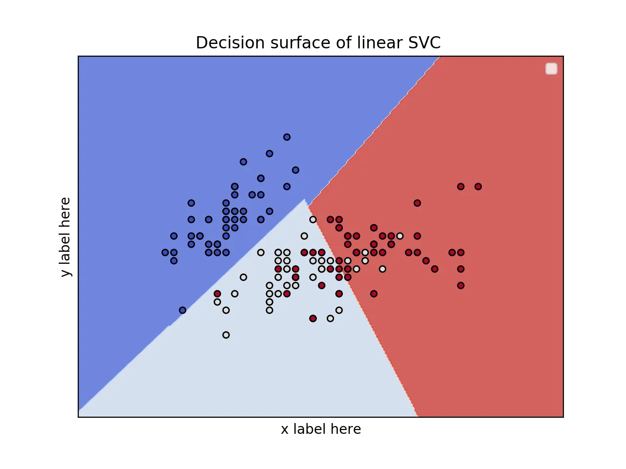
使用鸢尾花数据集的2D图表from sklearn.svm import SVC
import numpy as np
import matplotlib.pyplot as plt
from sklearn import svm, datasets
iris = datasets.load_iris()
X = iris.data[:, :2]
y = iris.target
def make_meshgrid(x, y, h=.02):
x_min, x_max = x.min() - 1, x.max() + 1
y_min, y_max = y.min() - 1, y.max() + 1
xx, yy = np.meshgrid(np.arange(x_min, x_max, h), np.arange(y_min, y_max, h))
return xx, yy
def plot_contours(ax, clf, xx, yy, **params):
Z = clf.predict(np.c_[xx.ravel(), yy.ravel()])
Z = Z.reshape(xx.shape)
out = ax.contourf(xx, yy, Z, **params)
return out
model = svm.SVC(kernel='linear')
clf = model.fit(X, y)
fig, ax = plt.subplots()
title = ('Decision surface of linear SVC ')
X0, X1 = X[:, 0], X[:, 1]
xx, yy = make_meshgrid(X0, X1)
plot_contours(ax, clf, xx, yy, cmap=plt.cm.coolwarm, alpha=0.8)
ax.scatter(X0, X1, c=y, cmap=plt.cm.coolwarm, s=20, edgecolors='k')
ax.set_ylabel('y label here')
ax.set_xlabel('x label here')
ax.set_xticks(())
ax.set_yticks(())
ax.set_title(title)
ax.legend()
plt.show()
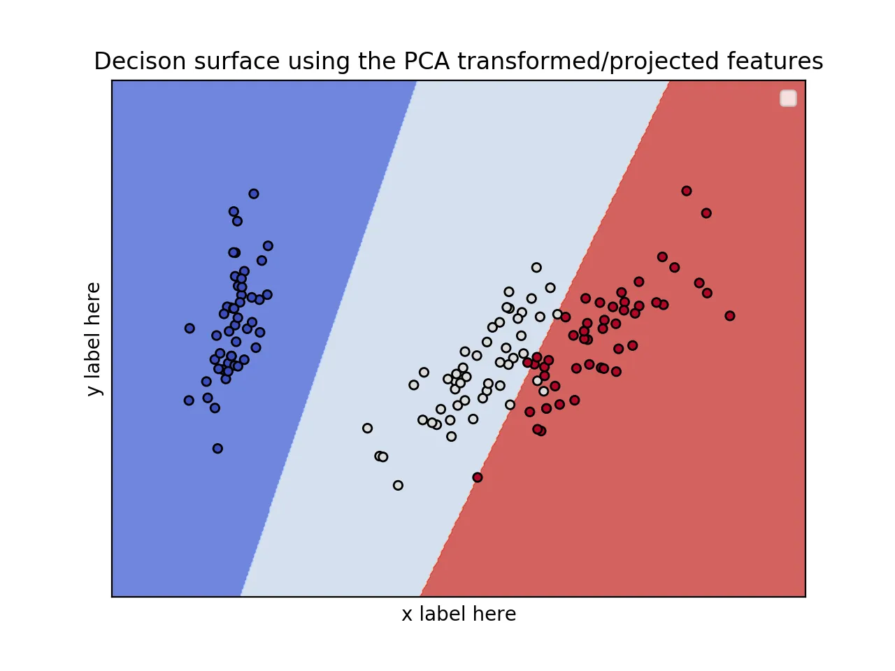
编辑:应用PCA降低维度。
from sklearn.svm import SVC
import numpy as np
import matplotlib.pyplot as plt
from sklearn import svm, datasets
from sklearn.decomposition import PCA
iris = datasets.load_iris()
X = iris.data
y = iris.target
pca = PCA(n_components=2)
Xreduced = pca.fit_transform(X)
def make_meshgrid(x, y, h=.02):
x_min, x_max = x.min() - 1, x.max() + 1
y_min, y_max = y.min() - 1, y.max() + 1
xx, yy = np.meshgrid(np.arange(x_min, x_max, h), np.arange(y_min, y_max, h))
return xx, yy
def plot_contours(ax, clf, xx, yy, **params):
Z = clf.predict(np.c_[xx.ravel(), yy.ravel()])
Z = Z.reshape(xx.shape)
out = ax.contourf(xx, yy, Z, **params)
return out
model = svm.SVC(kernel='linear')
clf = model.fit(Xreduced, y)
fig, ax = plt.subplots()
title = ('Decision surface of linear SVC ')
X0, X1 = Xreduced[:, 0], Xreduced[:, 1]
xx, yy = make_meshgrid(X0, X1)
plot_contours(ax, clf, xx, yy, cmap=plt.cm.coolwarm, alpha=0.8)
ax.scatter(X0, X1, c=y, cmap=plt.cm.coolwarm, s=20, edgecolors='k')
ax.set_ylabel('PC2')
ax.set_xlabel('PC1')
ax.set_xticks(())
ax.set_yticks(())
ax.set_title('Decison surface using the PCA transformed/projected features')
ax.legend()
plt.show()
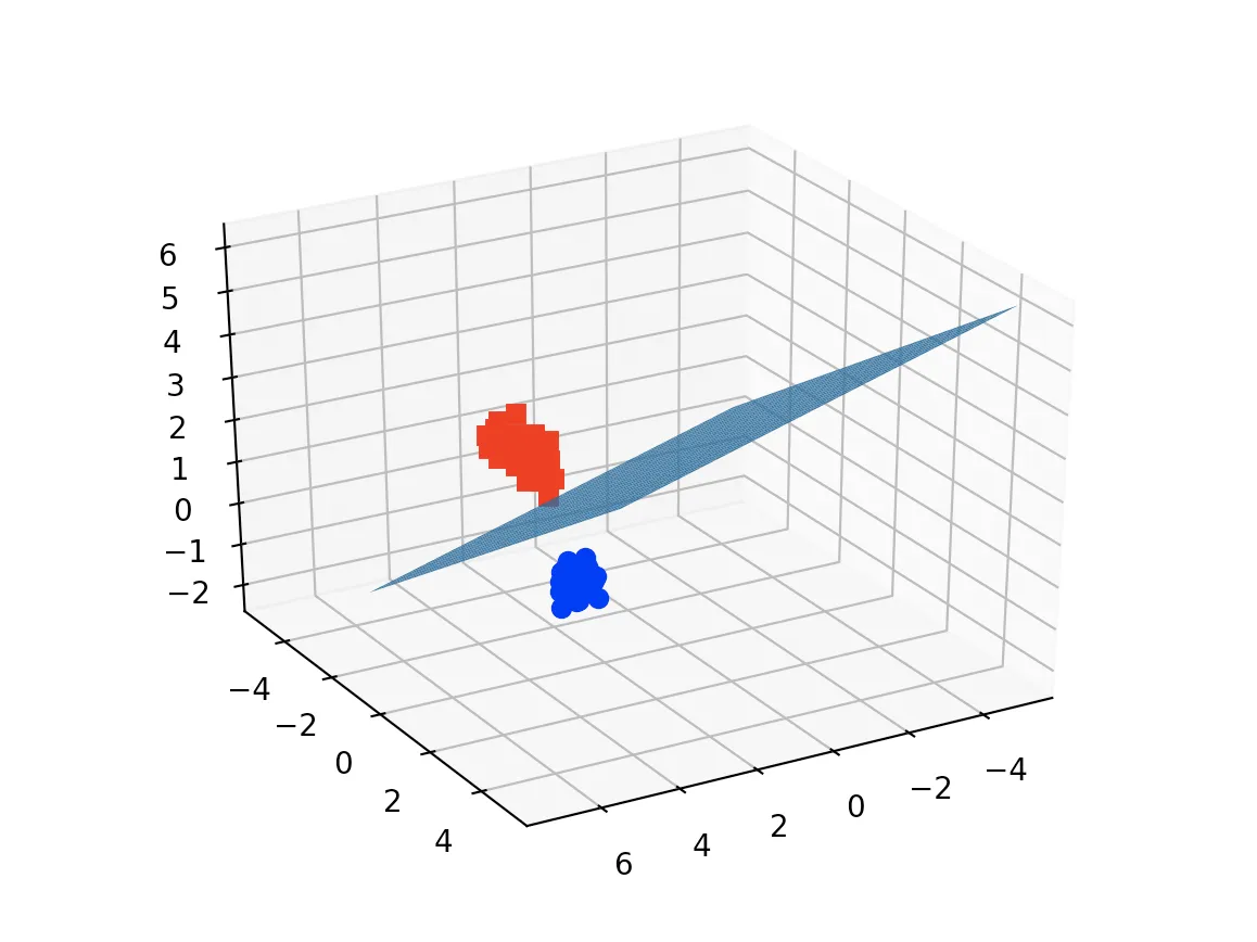
编辑1(2020年4月15日):
案例:使用鸢尾花数据集进行三个特征的3D图绘制
from sklearn.svm import SVC
import numpy as np
import matplotlib.pyplot as plt
from sklearn import svm, datasets
from mpl_toolkits.mplot3d import Axes3D
iris = datasets.load_iris()
X = iris.data[:, :3]
Y = iris.target
X = X[np.logical_or(Y==0,Y==1)]
Y = Y[np.logical_or(Y==0,Y==1)]
model = svm.SVC(kernel='linear')
clf = model.fit(X, Y)
z = lambda x,y: (-clf.intercept_[0]-clf.coef_[0][0]*x -clf.coef_[0][1]*y) / clf.coef_[0][2]
tmp = np.linspace(-5,5,30)
x,y = np.meshgrid(tmp,tmp)
fig = plt.figure()
ax = fig.add_subplot(111, projection='3d')
ax.plot3D(X[Y==0,0], X[Y==0,1], X[Y==0,2],'ob')
ax.plot3D(X[Y==1,0], X[Y==1,1], X[Y==1,2],'sr')
ax.plot_surface(x, y, z(x,y))
ax.view_init(30, 60)
plt.show()
sklearn.inspection.DecisionBoundaryDisplay,绘制VotingClassifier的决策边界,绘制在鸢尾花数据集上训练的决策树的决策面。 - Trenton McKinney