我需要一些提示来帮助我绘制决策边界,将数据分为两类。我使用Python NumPy创建了一些样本数据(来自高斯分布)。在这种情况下,每个数据点都是一个二维坐标,即一个由2行组成的1列向量。例如:
[ 1
  2 ]
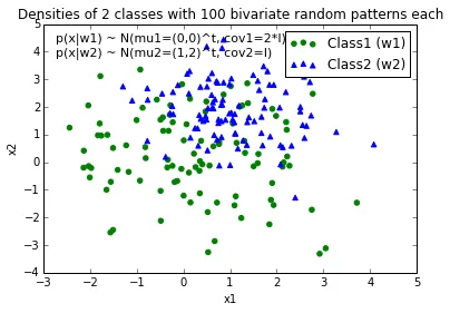
假设我有两个类,class1和class2,我通过下面的代码(分配给变量x1_samples和x2_samples)创建了100个class1数据点和100个class2数据点。
mu_vec1 = np.array([0,0])
cov_mat1 = np.array([[2,0],[0,2]])
x1_samples = np.random.multivariate_normal(mu_vec1, cov_mat1, 100)
mu_vec1 = mu_vec1.reshape(1,2).T # to 1-col vector

mu_vec2 = np.array([1,2])
cov_mat2 = np.array([[1,0],[0,1]])
x2_samples = np.random.multivariate_normal(mu_vec2, cov_mat2, 100)
mu_vec2 = mu_vec2.reshape(1,2).T
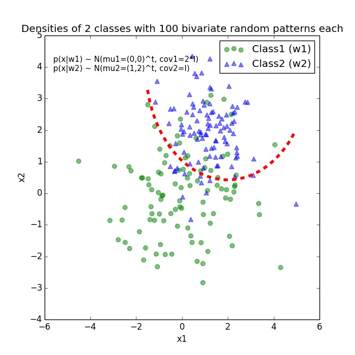
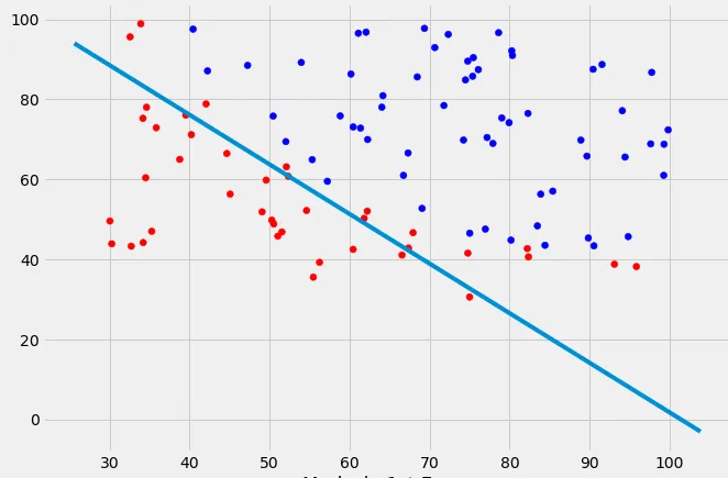
当我为每个类绘制数据点时,它看起来像这样:
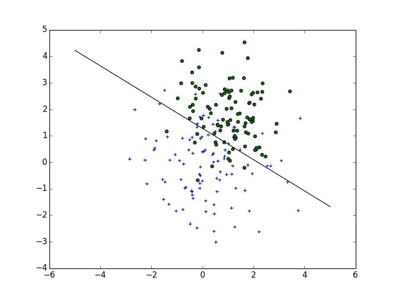
 现在,我想出了一个方程,用于将决策边界分离两个类,并希望将其添加到绘图中。但是,我不太确定如何绘制这个函数。
def decision_boundary(x_vec, mu_vec1, mu_vec2):
    g1 = (x_vec-mu_vec1).T.dot((x_vec-mu_vec1))
    g2 = 2*( (x_vec-mu_vec2).T.dot((x_vec-mu_vec2)) )
    return g1 - g2
我真的很感激任何帮助!
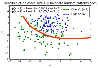
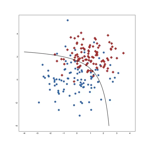
编辑: 如果我算对了的话,直觉上我会期望在绘制函数时决策边界看起来像这条红线...

 使用
使用 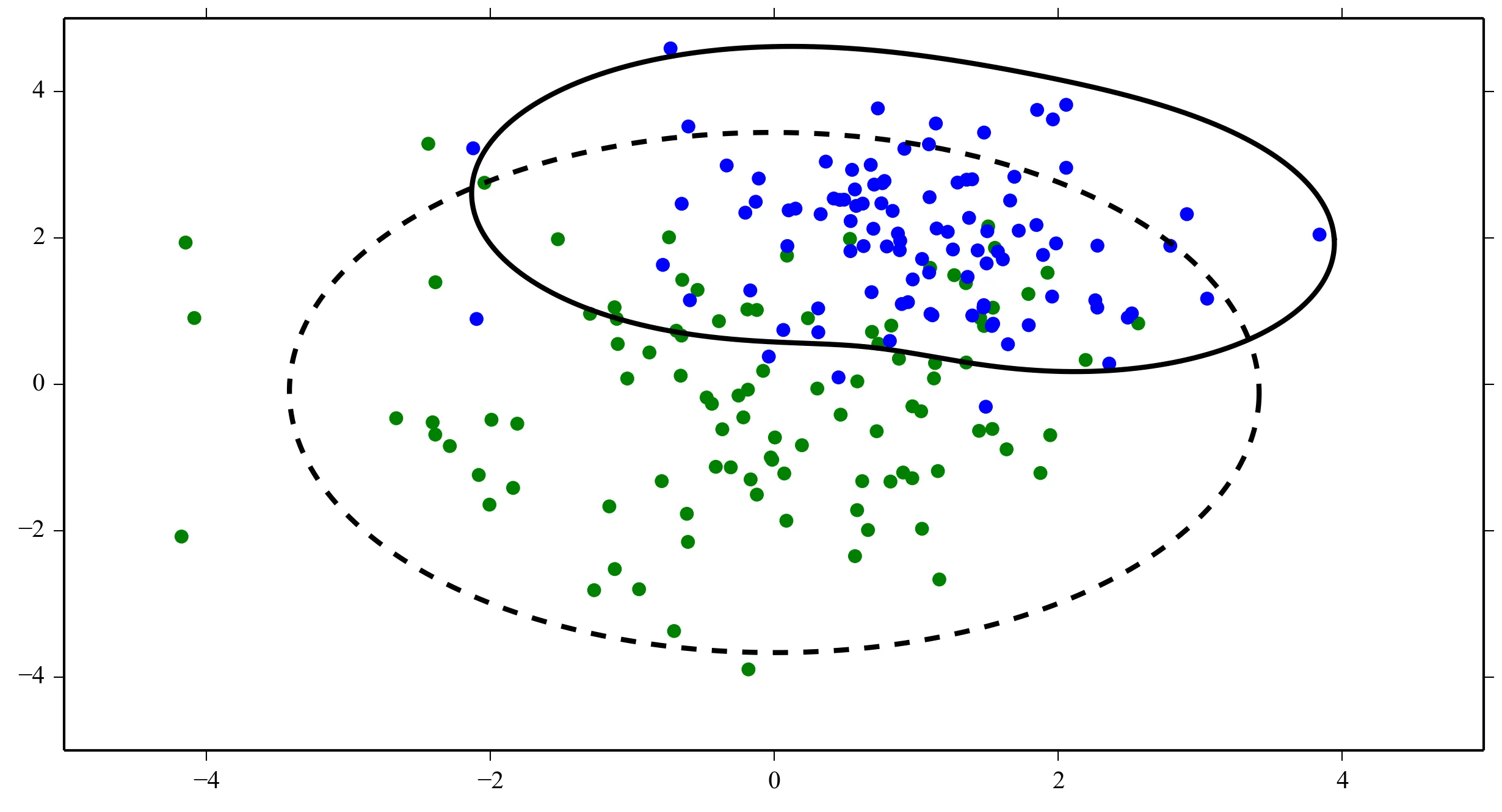 使用
使用  使用
使用 
 )
)
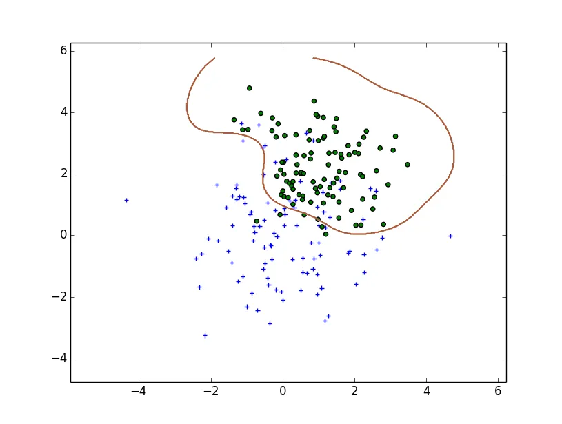
decision_boundary函数中的x_vec应该是什么?你只是想绘制一个分隔两个类别的线吗? - juniper-decision_boundary的0等高线。最简单的方法是在一个常规网格上评估函数并轮廓化结果。希望这能让你朝着正确的方向前进! - Joe Kington