将旋转矩阵应用于xy坐标

Question

我有一个代表给定空间中主题的xy坐标。它是参照另一个点并因此偏离中心。就像经度轴不沿着x轴对齐一样。

下面随机生成的椭圆提供了这方面的指示：

import numpy as np
from matplotlib.pyplot import scatter

xx = np.array([-0.51, 51.2])
yy = np.array([0.33, 51.6])
means = [xx.mean(), yy.mean()]  
stds = [xx.std() / 3, yy.std() / 3]
corr = 0.8         # correlation
covs = [[stds[0]**2          , stds[0]*stds[1]*corr], 
    [stds[0]*stds[1]*corr,           stds[1]**2]] 

m = np.random.multivariate_normal(means, covs, 1000).T
scatter(m[0], m[1])

为了将坐标“straighten”，我考虑应用矢量到一个旋转矩阵中。像这样的东西会有帮助吗？

angle = 65.
theta = (angle/180.) * np.pi

rotMatrix = np.array([[np.cos(theta), -np.sin(theta)], 
                     [np.sin(theta),  np.cos(theta)]])

这可能看起来是个愚蠢的问题，但有没有办法确定结果为 xy 坐标的向量是否垂直？或者你只能尝试调整旋转角度吗？

- user9639519

---

请查看我的答案上的第2次编辑，让我知道它是否适用于您。谢谢！ - b-fg

Answer 1

你可以使用 sklearn.decomposition.PCA（主成分分析）并设置 n_components=2，以提取旋转点云所需的最小角度，使其主轴水平。

可运行示例

import numpy as np
import matplotlib.pyplot as plt
from sklearn.decomposition import PCA

np.random.seed(1)

xx = np.array([-0.51, 51.2])
yy = np.array([0.33, 51.6])
means = [xx.mean(), yy.mean()]  
stds = [xx.std() / 3, yy.std() / 3]
corr = 0.8         # correlation
covs = [[stds[0]**2,       stds[0]*stds[1]*corr], 
        [stds[0]*stds[1]*corr, stds[1]**2]]

m = np.random.multivariate_normal(means, covs, 1000)

pca = PCA(2)

# This was in my first answer attempt: fit_transform works fine, but it randomly 
# flips (mirrors) points across one of the principal axes.
# m2 = pca.fit_transform(m)

# Workaround: get the rotation angle from the PCA components and manually 
# build the rotation matrix.

# Fit the PCA object, but do not transform the data
pca.fit(m)

# pca.components_ : array, shape (n_components, n_features)
# cos theta
ct = pca.components_[0, 0]
# sin theta
st = pca.components_[0, 1]

# One possible value of theta that lies in [0, pi]
t = np.arccos(ct)

# If t is in quadrant 1, rotate CLOCKwise by t
if ct > 0 and st > 0:
    t *= -1
# If t is in Q2, rotate COUNTERclockwise by the complement of theta
elif ct < 0 and st > 0:
    t = np.pi - t
# If t is in Q3, rotate CLOCKwise by the complement of theta
elif ct < 0 and st < 0:
    t = -(np.pi - t)
# If t is in Q4, rotate COUNTERclockwise by theta, i.e., do nothing
elif ct > 0 and st < 0:
    pass

# Manually build the ccw rotation matrix
rotmat = np.array([[np.cos(t), -np.sin(t)], 
                   [np.sin(t),  np.cos(t)]])

# Apply rotation to each row of m
m2 = (rotmat @ m.T).T

# Center the rotated point cloud at (0, 0)
m2 -= m2.mean(axis=0)

fig, ax = plt.subplots()
plot_kws = {'alpha': '0.75',
            'edgecolor': 'white',
            'linewidths': 0.75}
ax.scatter(m[:, 0], m[:, 1], **plot_kws)
ax.scatter(m2[:, 0], m2[:, 1], **plot_kws)

输出

警告: pca.fit_transform() 有时会翻转（镜像）点云

主成分可能随机出现为正或负。在某些情况下，您的点云可能会被翻转或甚至沿其主轴之一镜像。 （要测试这一点，请更改随机种子并重新运行代码，直到观察到翻转。）这里有一个深入讨论here（基于R，但数学相关）。要纠正这个问题，您需要用手动翻转一个或两个组件的符号替换fit_transform行，然后将符号翻转的组件矩阵乘以点云数组。

- Peter Leimbigler

---

感谢@Peter Leimbigler。这太棒了。我考虑了方向问题。只要所有点都按相同方向旋转，这不是一个大问题。例如，有些点被旋转了45度，而其他点被旋转了135度。你能确认一下吗？这样说通吗？ - user9639519

@Maxibon，我的原始代码可以随机地沿着其中一个主轴翻转（镜像）点云，这种情况下，并非每个点都会旋转相同的角度。我已经编辑了我的答案，包括手动修正，无论点云的原始方向如何，都应该最多旋转90º。 - Peter Leimbigler

Answer 2

在这里非常有用的概念是由矩阵 A 执行的向量 v 的线性变换。如果你把你的散点看作从 (0,0) 起始的向量的顶点，那么旋转它们到任意角度 theta 就非常容易了。一个执行这种旋转的角度为theta 的矩阵是：

A = [[cos(theta) -sin(theta]
     [sin(theta)  cos(theta)]]

显然，当θ角度为90度时，会导致

A = [[ 0 1]
     [-1 0]]

为了应用旋转，您只需要执行矩阵乘法w = A v

因此，当前目标是将存储在m中的向量与x、y坐标点m [0]，m [1]进行矩阵乘法运算，旋转后的向量将存储在m2中。以下是相关代码。请注意，我已经转置了m以便更轻松地计算矩阵乘法（使用@进行计算），而旋转角度为逆时针90度。

import numpy as np
import matplotlib.pyplot as plt

xx = np.array([-0.51, 51.2])
yy = np.array([0.33, 51.6])
means = [xx.mean(), yy.mean()]  
stds = [xx.std() / 3, yy.std() / 3]
corr = 0.8         # correlation
covs = [[stds[0]**2          , stds[0]*stds[1]*corr], 
    [stds[0]*stds[1]*corr,           stds[1]**2]] 

m = np.random.multivariate_normal(means, covs, 1000).T
plt.scatter(m[0], m[1])

theta_deg = 90
theta_rad = np.deg2rad(theta_deg)
A = np.matrix([[np.cos(theta_rad), -np.sin(theta_rad)],
               [np.sin(theta_rad), np.cos(theta_rad)]])
m2 = np.zeros(m.T.shape)

for i,v in enumerate(m.T):
  w = A @ v.T
  m2[i] = w
m2 = m2.T

plt.scatter(m2[0], m2[1])

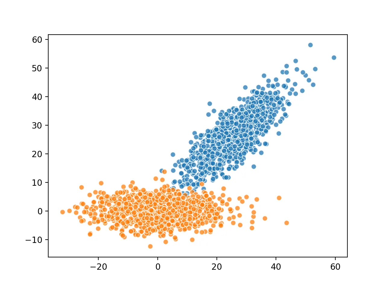
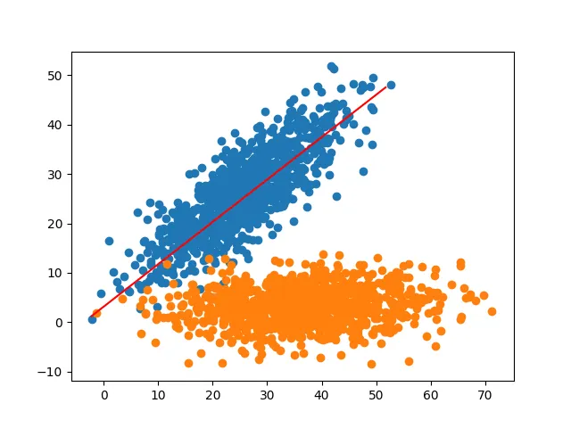
这导致了旋转的散点图： 通过线性变换，您可以确保旋转版本恰好逆时针旋转90度。 编辑 要找到旋转角度，使散点图与x轴对齐的方法是使用numpy.polyfit找到散点数据的线性近似。这会提供y轴截距b和slope的线性函数。然后使用arctan函数获取斜率的旋转角度，并像之前一样计算变换矩阵。您可以通过将以下部分添加到代码中来执行此操作。

slope, b = np.polyfit(m[1], m[0], 1)
x = np.arange(min(m[0]), max(m[0]), 1)
y_line = slope*x + b
plt.plot(x, y_line, color='r')
theta_rad = -np.arctan(slope)

并得到您正在寻找的图形结果

编辑2

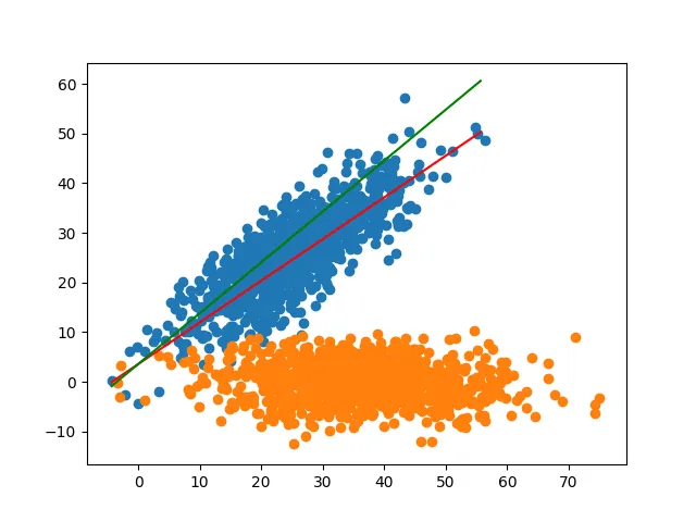
由于@Peter Leimbigler指出numpy.polyfit无法找到散点数据的正确全局方向，因此我想您可以通过平均数据的x和y部分来获得平均斜率。这是为了找到另一个斜率，称为slope2（现在以绿色表示）以应用旋转。所以简单地说，

slope, b = np.polyfit(m[1], m[0], 1)
x = np.arange(min(m[0]), max(m[0]), 1)
y_line = slope*x + b
slope2 = np.mean(m[1])/np.mean(m[0])
y_line2 = slope2*x + b
plt.plot(x, y_line, color='r')
plt.plot(x, y_line2, color='g')
theta_rad = -np.arctan(slope2)

通过使用旋转矩阵进行线性变换，您可以得到以下结果：

- b-fg

---

那么，您如何知道您需要 -45° 旋转而不是 -47° 呢？这就是问题所问的，如果我理解正确的话。 - ImportanceOfBeingErnest

是的，现在它似乎回答了这个问题。 - ImportanceOfBeingErnest

谢谢@b-fg。我以为我已经接受了之前的答案，抱歉。 - user9639519

@ImportanceOfBeingErnest，拟合椭圆可能有效，但我预计链接方法在这种密度最高的点云案例中会失败，并且边缘会逐渐变稀疏。那个拟合椭圆的代码是为已经大致沿着椭圆曲线的点设计的，而不是一个整体形状为椭圆的点簇。 - Peter Leimbigler

可以使用scipy.odr来拟合“总最小二乘”或“正交最小二乘”直线到数据中，但是PCA（或SVD）已经完全实现了这一点，并且据我所知，是找到椭圆点云的主轴与特征空间轴（例如+x轴）之间夹角问题的最正确和自然的解决方案。 - Peter Leimbigler

Answer 3

如果两条直线的斜率相乘等于-1，则它们互相垂直。 另一种情况是，当一条直线的斜率为0，另一条直线的斜率未定义时（即一条完全水平的直线和一条完全垂直的直线），也满足这个条件。

- DMarczak