如何在二维图上绘制 $\alpha$ 置信区间?

7

关于绘制置信区间有很多答案。

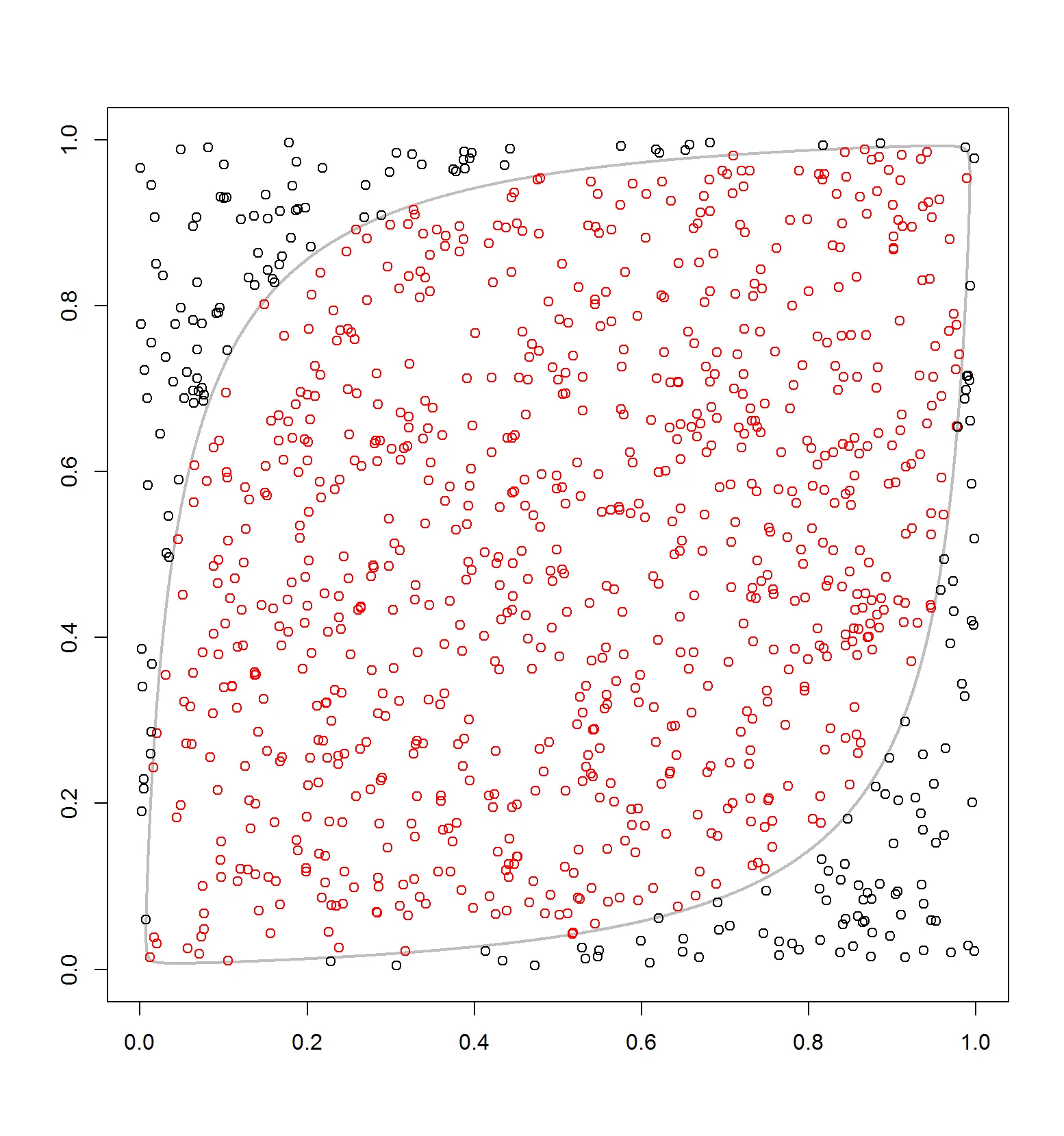
我正在阅读Lourme A. et al (2016)的论文,我想像该论文中的图2一样绘制90%置信边界和10%异常点:
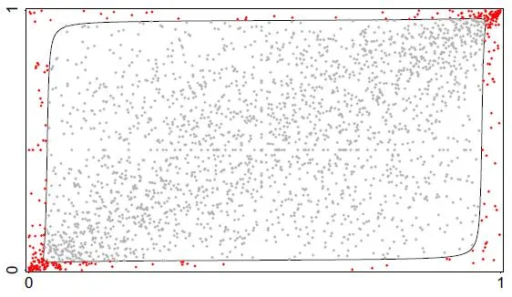
enter image description here

我不能使用LaTeX并插入定义置信区域的图片: enter image description here

library("MASS")
library(copula)
set.seed(612)

n <- 1000 # length of sample
d <- 2    # dimension

# random vector with uniform margins on (0,1)
u1 <- runif(n, min = 0, max = 1)
u2 <- runif(n, min = 0, max = 1)

u = matrix(c(u1, u2), ncol=d)

Rg  <- cor(u)   # d-by-d correlation matrix
Rg1 <- ginv(Rg) # inv. matrix 

# round(Rg %*% Rg1, 8) # check

# the multivariate c.d.f of u is a Gaussian copula 
# with parameter Rg[1,2]=0.02876654

normal.cop = normalCopula(Rg[1,2], dim=d)
fit.cop    = fitCopula(normal.cop, u, method="itau") #fitting
# Rg.hat     = fit.cop@estimate[1]
# [1] 0.03097071
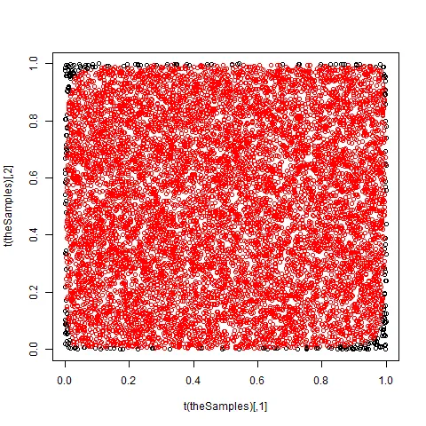
sim        = rCopula(n, normal.cop) # in (0,1)

# Taking the quantile function of N1(0, 1)

y1 <- qnorm(sim[,1], mean = 0, sd = 1)
y2 <- qnorm(sim[,2], mean = 0, sd = 1)

par(mfrow=c(2,2))

plot(y1, y2, col="red");  abline(v=mean(y1), h=mean(y2))
plot(sim[,1], sim[,2], col="blue")
hist(y1); hist(y2)

参考文献。Lourme, A.,F. Maurer(2016)在风险管理框架中测试高斯和学生t簇的方法。经济建模。
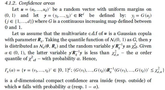
问题。 有人可以帮助我解释方程中变量v =(v_1,...,v_d)G(v_1),...,G(v_d)吗?

我认为v是非随机矩阵,其尺寸应为$k^2$(网格点)乘以d = 2(维度)。例如,

axis_x <- seq(0, 1, 0.1) # 11 grid points
axis_y <- seq(0, 1, 0.1) # 11 grid points
v <- expand.grid(axis_x, axis_y)
plot(v,  type = "p")

2
你是如何从数据点中定义这个“alpha”置信边界的? - Spacedman
2
信心总是与估计相关。你在估计什么? - Roland
1
所以你没有任何计算边界多边形的代码?这是你的第一个问题?你的第二个问题是绘制它吗? - Spacedman
1
@Nick,通常我们可以迁移,但由于赏金的原因我们无法这样做。 - Axeman
1
这篇文章 https://www.r-bloggers.com/copulas-made-easy/ 有帮助吗? - Drey
显示剩余9条评论
2个回答

4

所以,你的问题是关于向量nu和相应的G(nu)

nu是从具有区间(0,1)的任何分布中简单随机抽取的向量。(这里我使用均匀分布)。由于你希望样本在2D中,一个单一的nu可以是nu = runif(2)。根据上述解释,G是一个具有均值为0和协方差矩阵Rg的高斯概率密度函数。(在2D中,Rg的维数为2x2)。

现在这段话的意思是:如果你有一个随机样本nu,并且你希望它在给定维数d和置信水平alpha的情况下来自于Gamma,那么你需要计算以下统计量(G(nu) %*% Rg^-1) %*% G(nu),并检查它是否低于dalpha的Chi^2分布的概率密度函数。

例如:

# This is the copula parameter
Rg <- matrix(c(1,runif(2),1), ncol = 2)
# But we need to compute the inverse for sampling
Rginv <- MASS::ginv(Rg)

sampleResult <- replicate(10000, {
  # we draw our nu from uniform, but others that map to (0,1), e.g. beta, are possible, too
  nu <- runif(2)
  # we compute G(nu) which is a gaussian cdf on the sample
  Gnu <- qnorm(nu, mean = 0, sd = 1)
  # for this we compute the statistic as given in formula
  stat <- (Gnu %*% Rginv) %*% Gnu
  # and return the result
  list(nu = nu, Gnu = Gnu, stat = stat)
})

theSamples <- sapply(sampleResult["nu",], identity)

# this is the critical value of the Chi^2 with alpha = 0.95 and df = number of dimensions
# old and buggy threshold <- pchisq(0.95, df = 2)
# new and awesome - we are looking for the statistic at alpha = .95 quantile
threshold <- qchisq(0.95, df = 2)
# we can accept samples given the threshold (like in equation)
inArea <- sapply(sampleResult["stat",], identity) < threshold

plot(t(theSamples), col = as.integer(inArea)+1)

红点是您需要保留的点(我在此处绘制了所有点)。

enter image description here

关于绘制决策边界,我认为这有点复杂,因为您需要计算精确的 nu 对,以便 (Gnu %*% Rginv) %*% Gnu == pchisq(alpha, df = 2)。这是一个线性系统,你需要解出 Gnu 并应用反转来得到决策边界处的 nu编辑:重新阅读段落后,我注意到,Gnu 的参数不会改变,它只是 Gnu <- qnorm(nu, mean = 0, sd = 1)编辑:存在一个错误:对于阈值,您需要使用分位函数 qchisq 而不是分布函数 pchisq - 现在已在上面的代码中进行了更正(并更新了图表)。

注意事项:上述代码与论文中的说明非常相似。然而,结果并不完全对应于论文 - 置信区间是不同的,即sum(inArea)/length(inArea)alpha不接近。 - Drey
谢谢你的回答。我已经点赞了。我看到命令中 sd 的值是关键点:Gnu <- qnorm(nu, mean = 0, sd = .25)。根据论文,我们应该将 sd 设置为 1.0,但置信区间不同。我尝试计算 mean(sapply(sampleResult["stat",], identity)); sd(sapply(sampleResult["stat",], identity)); hist(sapply(sampleResult["stat",], identity)); 但我不知道如何指定 sd,以便置信区间接近 alpha。 - Nick
啊,阈值计算中有一个bug - 你需要使用qchisq而不是pchisq - 我已经在上面添加了解释。 - Drey

1
这有两个部分:首先,根据X和Y计算Copula值;然后,绘制曲线以给出Copula超过阈值的边界。
计算值基本上是线性代数,@drey已经回答了。这是一个重写版本,使Copula由函数给出。
cop1 <- function(x)
{
    Gnu <- qnorm(x)
    Gnu %*% Rginv %*% Gnu
}

copula <- function(x)
{
    apply(x, 1, cop1)
}

绘制边界曲线可以使用与此处相同的方法(这也是教科书《现代应用统计学》和《统计学习的要素》所使用的方法)。创建一个值网格,并使用插值来找到给定高度处的等高线。

Rg <- matrix(c(1,runif(2),1), ncol = 2)
Rginv <- MASS::ginv(Rg)

# draw the contour line where value == threshold
# define a grid of values first: avoid x and y = 0 and 1, where infinities exist
xlim <- 1e-3
delta <- 1e-3
xseq <- seq(xlim, 1-xlim, by=delta)
grid <- expand.grid(x=xseq, y=xseq)
prob.grid <- copula(grid)
threshold <- qchisq(0.95, df=2)

contour(x=xseq, y=xseq, z=matrix(prob.grid, nrow=length(xseq)), levels=threshold,
        col="grey", drawlabels=FALSE, lwd=2)

# add some points
data <- data.frame(x=runif(1000), y=runif(1000))
points(data, col=ifelse(copula(data) < threshold, "red", "black"))

enter image description here


网页内容由stack overflow 提供, 点击上面的
可以查看英文原文,
原文链接