Python中的高斯拟合

36

我试图针对我的数据(已经是一个粗略的高斯分布)拟合一个高斯分布曲线。我已经采纳了这里提供的建议并尝试了curve_fitleastsq,但我认为我缺少更基础的东西(因为我不知道如何使用这个命令)。 以下是我目前的脚本:

import pylab as plb
import matplotlib.pyplot as plt

# Read in data -- first 2 rows are header in this example. 
data = plb.loadtxt('part 2.csv', skiprows=2, delimiter=',')

x = data[:,2]
y = data[:,3]
mean = sum(x*y)
sigma = sum(y*(x - mean)**2)

def gauss_function(x, a, x0, sigma):
    return a*np.exp(-(x-x0)**2/(2*sigma**2))
popt, pcov = curve_fit(gauss_function, x, y, p0 = [1, mean, sigma])
plt.plot(x, gauss_function(x, *popt), label='fit')

# plot data

plt.plot(x, y,'b')

# Add some axis labels

plt.legend()
plt.title('Fig. 3 - Fit for Time Constant')
plt.xlabel('Time (s)')
plt.ylabel('Voltage (V)')
plt.show()

我从中得到的是一个类似高斯形状的曲线,这是我的原始数据,还有一条水平直线。

输入图片描述

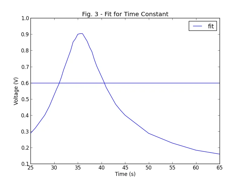
另外,我想用点来绘制我的图表,而不是把它们连接起来。 感谢任何意见!
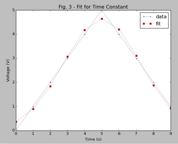

3
你缺少一些导入。mean 是乘积的总和,因此需要除以 len(x) - Steve Barnes
7个回答

37

这里是更正后的代码:

import pylab as plb
import matplotlib.pyplot as plt
from scipy.optimize import curve_fit
from scipy import asarray as ar,exp

x = ar(range(10))
y = ar([0,1,2,3,4,5,4,3,2,1])

n = len(x)                          #the number of data
mean = sum(x*y)/n                   #note this correction
sigma = sum(y*(x-mean)**2)/n        #note this correction

def gaus(x,a,x0,sigma):
    return a*exp(-(x-x0)**2/(2*sigma**2))

popt,pcov = curve_fit(gaus,x,y,p0=[1,mean,sigma])

plt.plot(x,y,'b+:',label='data')
plt.plot(x,gaus(x,*popt),'ro:',label='fit')
plt.legend()
plt.title('Fig. 3 - Fit for Time Constant')
plt.xlabel('Time (s)')
plt.ylabel('Voltage (V)')
plt.show()

结果:
这里输入图片描述


如果您使用 plt.plot(x,y,'b+',label='data'),它们将只是点。 - Developer
2
这个答案没有解释为什么更正后的定义比原始定义更好。 - strpeter
1
为了让它适用于不同的数据集,我添加了 yn = max(y)y /= yn,然后在绘图时,我将 y 更改为 y*ynplt.plot(x, y*yn, ...) - EL_DON
1
@开发者:我猜你想做的是除以sum(y)或等价的mean = np.average(x, weights=y),这相当于5.0。我问自己为什么要除以n,这会返回12.0——一个远离真实值的数值。在一般情况下,你甚至不能确定这是否收敛到正确的值,因为正确的做法是除以sum(y),而这可能远离n - strpeter
1
@HereItIs 拟合例程可能会在输入数据非常大(小)的情况下内部发生浮点溢出(下溢)。通常将数据标准化为最大输入值可以预防此问题。 - EL_DON
显示剩余4条评论

31

解释

您需要良好的起始值,以使curve_fit函数在“好”的值处收敛。我无法确切地说出为什么您的拟合没有收敛(即使您的平均值定义很奇怪-请查看下面),但是我将为您提供一种适用于类似于您的非归一化高斯函数的策略。

示例

估计参数应该接近最终值(使用加权算术平均数-除以所有值的和):

import matplotlib.pyplot as plt
from scipy.optimize import curve_fit
import numpy as np

x = np.arange(10)
y = np.array([0, 1, 2, 3, 4, 5, 4, 3, 2, 1])

# weighted arithmetic mean (corrected - check the section below)
mean = sum(x * y) / sum(y)
sigma = np.sqrt(sum(y * (x - mean)**2) / sum(y))

def Gauss(x, a, x0, sigma):
    return a * np.exp(-(x - x0)**2 / (2 * sigma**2))

popt,pcov = curve_fit(Gauss, x, y, p0=[max(y), mean, sigma])

plt.plot(x, y, 'b+:', label='data')
plt.plot(x, Gauss(x, *popt), 'r-', label='fit')
plt.legend()
plt.title('Fig. 3 - Fit for Time Constant')
plt.xlabel('Time (s)')
plt.ylabel('Voltage (V)')
plt.show()

我个人更喜欢使用numpy。

对均值的定义发表评论(包括开发者的回答)

由于审稿人不喜欢我的#Developer 代码的编辑,我将解释在什么情况下建议改进代码。 开发者的平均值不符合均值的正常定义之一。

您的定义返回:

>>> sum(x * y)
125

开发者定义返回结果:

>>> sum(x * y) / len(x)
12.5 #for Python 3.x

加权算术平均值:

>>> sum(x * y) / sum(y)
5.0

同样地,您可以比较标准偏差(sigma)的定义。与得到的拟合图形进行比较:

Resulting fit

针对Python 2.x用户的说明

在Python 2.x中,您还应该使用新的除法以避免出现奇怪的结果或者在除法之前明确转换这些数字:

from __future__ import division

例如

sum(x * y) * 1. / sum(y)

我喜欢“加权算术平均数”。在某些情况下,它可以使均值和标准差的估计更加准确(例如,如果您有一个长的左尾和短的右尾)。然而,当我试图谷歌一下为什么“加权算术平均数”更好的理论解释时,我什么都没找到。这很奇怪... - halfmoonhalf
你看到维基百科的链接了吗?你也可以查找期望值的定义——这个值是从现有数据中最有可能再次出现的值。 - strpeter

6

如果没有收敛,你会得到一条水平直线。

如果将拟合的第一个参数(p0)设定为max(y)(在示例中为5),而不是1,就可以获得更好的收敛性。


4
在我花费数小时寻找错误后,发现问题出在你的公式上: sigma = sum(y*(x-mean)**2)/n 但是这个公式是错误的,正确的公式应该是它的平方根: sqrt(sum(y*(x-mean)**2)/n) 希望这可以帮到你。

2
还有一个错误:不是1/n而是1/sum(y)。请查看下面的答案 - strpeter

1
sigma = sum(y*(x - mean)**2)

应该是:

应该是

sigma = np.sqrt(sum(y*(x - mean)**2))

1
实际上,您不需要进行第一次猜测。只需执行
import matplotlib.pyplot as plt  
from scipy.optimize import curve_fit
from scipy import asarray as ar,exp

x = ar(range(10))
y = ar([0,1,2,3,4,5,4,3,2,1])

n = len(x)                          #the number of data
mean = sum(x*y)/n                   #note this correction
sigma = sum(y*(x-mean)**2)/n        #note this correction

def gaus(x,a,x0,sigma):
    return a*exp(-(x-x0)**2/(2*sigma**2))

popt,pcov = curve_fit(gaus,x,y)
#popt,pcov = curve_fit(gaus,x,y,p0=[1,mean,sigma])

plt.plot(x,y,'b+:',label='data')
plt.plot(x,gaus(x,*popt),'ro:',label='fit')
plt.legend()
plt.title('Fig. 3 - Fit for Time Constant')
plt.xlabel('Time (s)')
plt.ylabel('Voltage (V)')
plt.show()

运行正常。这更简单,因为猜测并不简单。我的数据更复杂,无法进行适当的第一次猜测,但是简单地删除第一个猜测就可以正常工作 :)

P.S.: scipy 中的警告建议使用 numpy.exp() 更好


1

网页内容由stack overflow 提供, 点击上面的
可以查看英文原文,
原文链接