我的问题简述如下:我有一些数据的直方图(行星密度),似乎有三个峰值。现在我想将三个高斯函数拟合到这个直方图上。
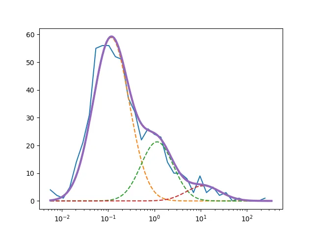
我期望得到以下结果: 我尝试使用不同的方法来拟合高斯函数:curve_fit、最小二乘法和sklearn.mixture中的GaussianMixture。使用curve_fit可以得到一个相当好的拟合结果:
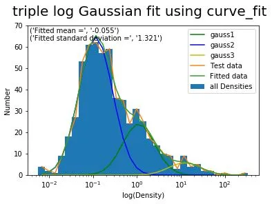 但是与期望的结果相比,还不够好。使用最小二乘法可以得到一个“良好的拟合”:
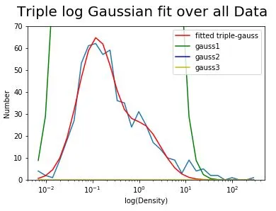
但我的高斯函数是无意义的,并且使用GaussianMixture无济于事,因为我无法将我看到的示例代码适应我的问题。
现在我有三个问题:
1. 最重要的问题:如何更好地拟合我的第三个高斯函数?我已经尝试调整初始值p0,但高斯函数会变得更糟或根本找不到参数。 2. 我的最小二乘法代码有什么问题?为什么它给我如此奇怪的高斯函数?是否有办法修复它?我的猜测是:它是否因为最小二乘法会尽力使拟合和实际数据之间的误差最小? 3. 我该如何使用GaussianMixture完成整个过程?我找到了这篇文章:
https://dev59.com/b1gR5IYBdhLWcg3wLa28
但是无法将其适应到我的问题上。
我真的想理解如何正确地进行拟合,因为在将来我将不得不经常这样做。问题是我对统计学不是很熟悉,并且刚刚开始使用Python编程。
以下是三种不同的代码:
Curvefit
我期望得到以下结果:
我尝试使用不同的方法来拟合高斯函数:curve_fit、最小二乘法和sklearn.mixture中的GaussianMixture。使用curve_fit可以得到一个相当好的拟合结果:
但是与期望的结果相比,还不够好。使用最小二乘法可以得到一个“良好的拟合”:
但我的高斯函数是无意义的,并且使用GaussianMixture无济于事,因为我无法将我看到的示例代码适应我的问题。
现在我有三个问题:
1. 最重要的问题:如何更好地拟合我的第三个高斯函数?我已经尝试调整初始值p0,但高斯函数会变得更糟或根本找不到参数。 2. 我的最小二乘法代码有什么问题?为什么它给我如此奇怪的高斯函数?是否有办法修复它?我的猜测是:它是否因为最小二乘法会尽力使拟合和实际数据之间的误差最小? 3. 我该如何使用GaussianMixture完成整个过程?我找到了这篇文章:
https://dev59.com/b1gR5IYBdhLWcg3wLa28
但是无法将其适应到我的问题上。
我真的想理解如何正确地进行拟合,因为在将来我将不得不经常这样做。问题是我对统计学不是很熟悉,并且刚刚开始使用Python编程。
以下是三种不同的代码:
Curvefit
import numpy as np
import math
import matplotlib.pyplot as plt
from scipy.optimize import curve_fit

hist, bin_edges = np.histogram(Density, bins=np.logspace(np.log10(MIN), np.log10(MAX), 32))

bin_centres = (bin_edges[:-1] + bin_edges[1:])/2

# Define model function to be used to fit to the data above:
def triple_gaussian(  x,*p ):
    (c1, mu1, sigma1, c2, mu2, sigma2, c3, mu3, sigma3) = p
    res =    np.divide(1,x)*c1 * np.exp( - (np.log(x) - mu1)**2.0 / (2.0 * sigma1**2.0) ) \
          +  np.divide(1,x)*c2 * np.exp( - (np.log(x) - mu2)**2.0 / (2.0 * sigma2**2.0) ) \
          +  np.divide(1,x)*c3 * np.exp( - (np.log(x) - mu3)**2.0 / (2.0 * sigma3**2.0) )
    return res

# p0 is the initial guess for the fitting coefficients (A, mu and sigma above)
p0 = [60., 1, 1., 30., 1., 1.,10., 1., 1]

coeff, var_matrix = curve_fit(triple_gaussian, bin_centres, hist, p0=p0)

# Get the fitted curve
hist_fit = triple_gaussian(bin_centres, *coeff)

c1 =coeff[0]
mu1 =coeff[1]
sigma1 =coeff[2]
c2 =coeff[3]
mu2 =coeff[4]
sigma2 =coeff[5]
c3 =coeff[6]
mu3 =coeff[7]
sigma3 =coeff[8]
x= bin_centres

gauss1= np.divide(1,x)*c1 * np.exp( - (np.log(x) - mu1)**2.0 / (2.0 * sigma1**2.0) )
gauss2= np.divide(1,x)*c2 * np.exp( - (np.log(x) - mu2)**2.0 / (2.0 * sigma2**2.0) )
gauss3= np.divide(1,x)*c3 * np.exp( - (np.log(x) - mu3)**2.0 / (2.0 * sigma3**2.0) )

plt.plot(x,gauss1, 'g',label='gauss1')
plt.plot(x,gauss2, 'b', label='gauss2')
plt.plot(x,gauss3, 'y', label='gauss3')
plt.gca().set_xscale("log")
plt.legend(loc='upper right')
plt.ylim([0,70])
plt.suptitle('Triple log Gaussian fit over all Data', fontsize=20)
plt.xlabel('log(Density)')
plt.ylabel('Number')

plt.hist(Density, bins=np.logspace(np.log10(MIN), np.log10(MAX), 32), label='all Densities')
plt.plot(bin_centres, hist, label='Test data')
plt.plot(bin_centres, hist_fit, label='Fitted data')
plt.gca().set_xscale("log")
plt.ylim([0,70])
plt.suptitle('triple log Gaussian fit using curve_fit', fontsize=20)
plt.xlabel('log(Density)')
plt.ylabel('Number')
plt.legend(loc='upper right')
plt.annotate(Text1, xy=(0.01, 0.95), xycoords='axes fraction')
plt.annotate(Text2, xy=(0.01, 0.90), xycoords='axes fraction')
plt.savefig('all Densities_gauss')
plt.show()
最小二乘法
拟合本身看起来还不错,但三个高斯曲线很糟糕。请参见下图:
    # I only have x-data, so to get according y-data I make my histogram and
 #use the bins as x-data and the numbers (hist) as y-data.
#Density is a Dataset of 581 Values between 0 and 340.

hist, bin_edges = np.histogram(Density, bins=np.logspace(np.log10(MIN), np.log10(MAX), 32))
x = (bin_edges[:-1] + bin_edges[1:])/2
y = hist

#define tripple gaussian

def triple_gaussian(  p,x ):
    (c1, mu1, sigma1, c2, mu2, sigma2, c3, mu3, sigma3) = p
    res =    np.divide(1,x)*c1 * np.exp( - (np.log(x) - mu1)**2.0 / (2.0 * sigma1**2.0) ) \
          +  np.divide(1,x)*c2 * np.exp( - (np.log(x) - mu2)**2.0 / (2.0 * sigma2**2.0) ) \
          +  np.divide(1,x)*c3 * np.exp( - (np.log(x) - mu3)**2.0 / (2.0 * sigma3**2.0) )
    return res

def errfunc(p,x,y):
   return y-triple_gaussian(p,x)

p0=[]
p0 = [60., 0.1, 1., 30., 1., 1.,10., 10., 1.]
fit = optimize.leastsq(errfunc,p0,args=(x,y))

print('fit', fit)


plt.plot(x,y)
plt.plot(x,triple_gaussian(fit[0],x), 'r')
plt.gca().set_xscale("log")
plt.ylim([0,70])
plt.suptitle('Double log Gaussian fit over all Data', fontsize=20)
plt.xlabel('log(Density)')
plt.ylabel('Number')

c1, mu1, sigma1, c2, mu2, sigma2, c3, mu3, sigma3=fit[0]

print('c1', c1)

gauss1= np.divide(1,x)*c1 * np.exp( - (np.log(x) - mu1)**2.0 / (2.0 * sigma1**2.0) )
gauss2= np.divide(1,x)*c2 * np.exp( - (np.log(x) - mu2)**2.0 / (2.0 * sigma2**2.0) )
gauss3= np.divide(1,x)*c3 * np.exp( - (np.log(x) - mu3)**2.0 / (2.0 * sigma3**2.0) )

plt.plot(x,gauss1, 'g')
plt.plot(x,gauss2, 'b')
plt.plot(x,gauss3, 'y')
plt.gca().set_xscale("log")
plt.ylim([0,70])
plt.suptitle('Double log Gaussian fit over all Data', fontsize=20)
plt.xlabel('log(Density)')
plt.ylabel('Number')
GaussianMixture
我之前说过,我并不真正理解 GaussianMixture。我不知道是否需要像之前那样定义 triplegauss,还是只需定义 gauss,GaussianMixture 就能自行发现其中有三个高斯分布。
我也不明白在哪里使用哪些数据,因为当我使用 bins 和 hist 值时,“拟合曲线”仅仅是连接在一起的数据点。所以我想我使用了错误的数据。
我不理解的部分是 #Fit GMM 和 #Construct function manually as sum of gaussians.
hist, bin_edges = np.histogram(Density, bins=np.logspace(np.log10(MIN), np.log10(MAX), 32))

bin_centres = (bin_edges[:-1] + bin_edges[1:])/2

plt.hist(Density, bins=np.logspace(np.log10(MIN), np.log10(MAX), 32), label='all Densities')
plt.gca().set_xscale("log")
plt.ylim([0,70])

# Define simple gaussian
def gauss_function(x, amp, x0, sigma):
    return np.divide(1,x)*amp * np.exp(-(np.log(x) - x0) ** 2. / (2. * sigma ** 2.))

# My Data
samples = Density

# Fit GMM
gmm = GaussianMixture(n_components=3, covariance_type="full", tol=0.00001)
gmm = gmm.fit(X=np.expand_dims(samples, 1))

gmm_x= bin_centres
gmm_y= hist
# Construct function manually as sum of gaussians
gmm_y_sum = np.full_like(gmm_x, fill_value=0, dtype=np.float32)
for m, c, w in zip(gmm.means_.ravel(), gmm.covariances_.ravel(), gmm.weights_.ravel()):
    gauss = gauss_function(x=gmm_x, amp=1, x0=m, sigma=np.sqrt(c))
    gmm_y_sum += gauss / np.trapz(gauss, gmm_x) *w

# Make regular histogram
fig, ax = plt.subplots(nrows=1, ncols=1, figsize=[8, 5])
ax.hist(samples, bins=np.logspace(np.log10(MIN), np.log10(MAX), 32), label='all Densities')
ax.plot(gmm_x, gmm_y, color="crimson", lw=4, label="GMM")
ax.plot(gmm_x, gmm_y_sum, color="black", lw=4, label="Gauss_sum", linestyle="dashed")
plt.gca().set_xscale("log")
plt.ylim([0,70])

# Annotate diagram
ax.set_ylabel("Probability density")
ax.set_xlabel("Arbitrary units")

# Make legend
plt.legend()

plt.show()
我希望有人能够至少回答我的一个问题。如我之前所说,如果有任何遗漏或需要更多信息,请告诉我。
提前感谢!
--编辑-- 这里是我的数据。