在R中实现梯度下降算法的基础上使用随机梯度下降算法

Question

在R中实现梯度下降算法的基础上使用随机梯度下降算法

10

我在R中实现了多元线性回归的梯度下降算法。我想看看是否可以使用现有的方法运行随机梯度下降算法。我不确定这是否真的是低效的。例如，对于每个α值，我想执行500次SGD迭代，并能够指定每次迭代中随机选择的样本数量。这样做将很好地展示样本数量对结果的影响。但是，我遇到了小批量处理的问题，并且希望能够轻松绘制结果。以下是我目前的进展：

 # Read and process the datasets

# download the files from GitHub
download.file("https://raw.githubusercontent.com/dbouquin/IS_605/master/sgd_ex_data/ex3x.dat", "ex3x.dat", method="curl")
x <- read.table('ex3x.dat')

# we can standardize the x vaules using scale()
x <- scale(x)

download.file("https://raw.githubusercontent.com/dbouquin/IS_605/master/sgd_ex_data/ex3y.dat", "ex3y.dat", method="curl")
y <- read.table('ex3y.dat')

# combine the datasets
data3 <- cbind(x,y)
colnames(data3) <- c("area_sqft", "bedrooms","price")
str(data3)

head(data3)

################ Regular Gradient Descent
# http://www.r-bloggers.com/linear-regression-by-gradient-descent/

# vector populated with 1s for the intercept coefficient
x1 <- rep(1, length(data3$area_sqft))

# appends to dfs
# create x-matrix of independent variables
x <- as.matrix(cbind(x1,x))
# create y-matrix of dependent variables
y <- as.matrix(y)
L <- length(y)

# cost gradient function: independent variables and values of thetas
cost <- function(x,y,theta){
  gradient <- (1/L)* (t(x) %*% ((x%*%t(theta)) - y))
  return(t(gradient)) 
}

# GD simultaneous update algorithm
# https://www.coursera.org/learn/machine-learning/lecture/8SpIM/gradient-descent
GD <- function(x, alpha){
      theta <- matrix(c(0,0,0), nrow=1) 
  for (i in 1:500) {
       theta <- theta - alpha*cost(x,y,theta)  
       theta_r <- rbind(theta_r,theta)    
  }
return(theta_r)
}

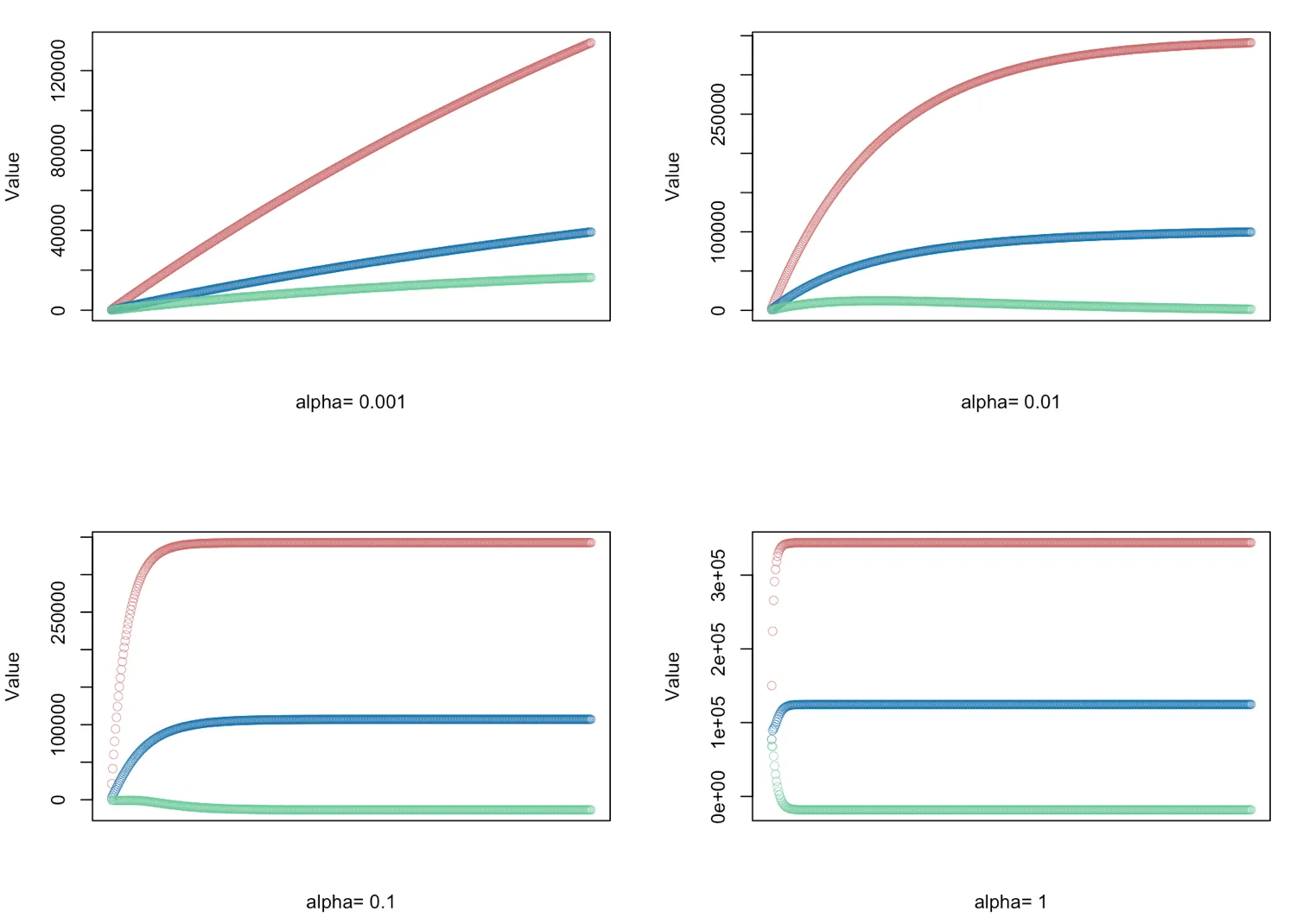
# gradient descent α = (0.001, 0.01, 0.1, 1.0) - defined for 500 iterations

alphas <- c(0.001,0.01,0.1,1.0)

# Plot price, area in square feet, and the number of bedrooms

# create empty vector theta_r
theta_r<-c()

for(i in 1:length(alphas)) {

 result <- GD(x, alphas[i])

 # red = price 
 # blue = sq ft 
 # green = bedrooms
 plot(result[,1],ylim=c(min(result),max(result)),col="#CC6666",ylab="Value",lwd=0.35,
      xlab=paste("alpha=", alphas[i]),xaxt="n") #suppress auto x-axis title
      lines(result[,2],type="b",col="#0072B2",lwd=0.35)
      lines(result[,3],type="b",col="#66CC99",lwd=0.35)
}

是否更实际找到使用sgd()的方法？我似乎无法通过sgd包获得我所寻求的控制水平。

- Daina

我会尝试一下，但是我在阅读sgd文档方面遇到了很多麻烦。如果可能的话，能够在我已有的基础上进行构建就太好了。你看过使用R中sgd进行多变量线性回归的任何演示或示例吗？我只找到了线性回归的内容。 - Daina

例如，我找到了这篇文章，但它并没有什么帮助。 - Daina

1

?sgd中有一个多变量线性示例，尽管它相当简单。还有一个vignette。 - rawr

嗯... 还没看过这篇论文呢。我得今天读一下 — 谢谢！ - alexwhitworth

1

检查源代码，model.control和sgd.control似乎由sgd:::valid_model_control和sgd:::valid_sgd_control控制，尽管我没有看到有关观测数量的选项。鉴于sgd在批量大小==1时保证最优，可能没有选项。通常，批量大小仅指定为控制学习时间（计算时间而不是迭代次数）...由于该软件包正在积极开发中，建议您与作者提出问题...即使您使用下面rawr的包装器。 - alexwhitworth

显示剩余3条评论

1个回答

网页内容由stack overflow 提供, 点击上面的

可以查看英文原文，
原文链接

- rawr · Accepted Answer

坚持现有的技术方案

## all of this is the same

download.file("https://raw.githubusercontent.com/dbouquin/IS_605/master/sgd_ex_data/ex3x.dat", "ex3x.dat", method="curl")
x <- read.table('ex3x.dat')
x <- scale(x)
download.file("https://raw.githubusercontent.com/dbouquin/IS_605/master/sgd_ex_data/ex3y.dat", "ex3y.dat", method="curl")
y <- read.table('ex3y.dat')
data3 <- cbind(x,y)
colnames(data3) <- c("area_sqft", "bedrooms","price")
x1 <- rep(1, length(data3$area_sqft))
x <- as.matrix(cbind(x1,x))
y <- as.matrix(y)
L <- length(y)
cost <- function(x,y,theta){
  gradient <- (1/L)* (t(x) %*% ((x%*%t(theta)) - y))
  return(t(gradient)) 
}

我在你的 GD 函数中添加了 y，并创建了一个包装函数 myGoD，在调用你的函数之前对数据进行子集处理。

GD <- function(x, y, alpha){
  theta <- matrix(c(0,0,0), nrow=1)
  theta_r <- NULL
  for (i in 1:500) {
    theta <- theta - alpha*cost(x,y,theta)  
    theta_r <- rbind(theta_r,theta)    
  }
  return(theta_r)
}

myGoD <- function(x, y, alpha, n = nrow(x)) {
  idx <- sample(nrow(x), n)
  y <- y[idx, , drop = FALSE]
  x <- x[idx, , drop = FALSE]
  GD(x, y, alpha)
}

请确认它是否可用，并尝试使用不同的 Ns

all.equal(GD(x, y, 0.001), myGoD(x, y, 0.001))
# [1] TRUE

set.seed(1)
head(myGoD(x, y, 0.001, n = 20), 2)
#          x1        V1       V2
# V1 147.5978  82.54083 29.26000
# V1 295.1282 165.00924 58.48424

set.seed(1)
head(myGoD(x, y, 0.001, n = 40), 2)
#          x1        V1        V2
# V1 290.6041  95.30257  59.66994
# V1 580.9537 190.49142 119.23446

以下是如何使用它的方法

alphas <- c(0.001,0.01,0.1,1.0)
ns <- c(47, 40, 30, 20, 10)

par(mfrow = n2mfrow(length(alphas)))
for(i in 1:length(alphas)) {

  # result <- myGoD(x, y, alphas[i]) ## original
  result <- myGoD(x, y, alphas[i], ns[i])

  # red = price 
  # blue = sq ft 
  # green = bedrooms
  plot(result[,1],ylim=c(min(result),max(result)),col="#CC6666",ylab="Value",lwd=0.35,
       xlab=paste("alpha=", alphas[i]),xaxt="n") #suppress auto x-axis title
  lines(result[,2],type="b",col="#0072B2",lwd=0.35)
  lines(result[,3],type="b",col="#66CC99",lwd=0.35)
}

您不需要包装函数 - 您可以稍微更改您的GD。显式传递参数到函数而不是依赖作用域始终是一个好习惯。在之前，您假设y将从全局环境中提取; 在这里，必须给出y，否则将出现错误。这将避免许多未来的头痛和错误。

GD <- function(x, y, alpha, n = nrow(x)){
  idx <- sample(nrow(x), n)
  y <- y[idx, , drop = FALSE]
  x <- x[idx, , drop = FALSE]
  theta <- matrix(c(0,0,0), nrow=1)
  theta_r <- NULL

  for (i in 1:500) {
    theta <- theta - alpha*cost(x,y,theta)  
    theta_r <- rbind(theta_r,theta)    
  }
  return(theta_r)
}