如何在Python中快速减少自相关函数的噪声？

Question

如何在Python中快速减少自相关函数的噪声？

4

我可以使用numpy的内置功能计算自相关： numpy.correlate(x,x,mode='same') 然而，所得到的相关性自然是有噪声的。我可以将数据分区，并在每个结果窗口上计算相关性，然后将它们全部平均起来以计算更干净的自相关，类似于signal.welch所做的。是否有一个方便的函数在numpy或scipy中可以做到这一点，可能比我自己计算分区并循环遍历数据得到的速度更快？

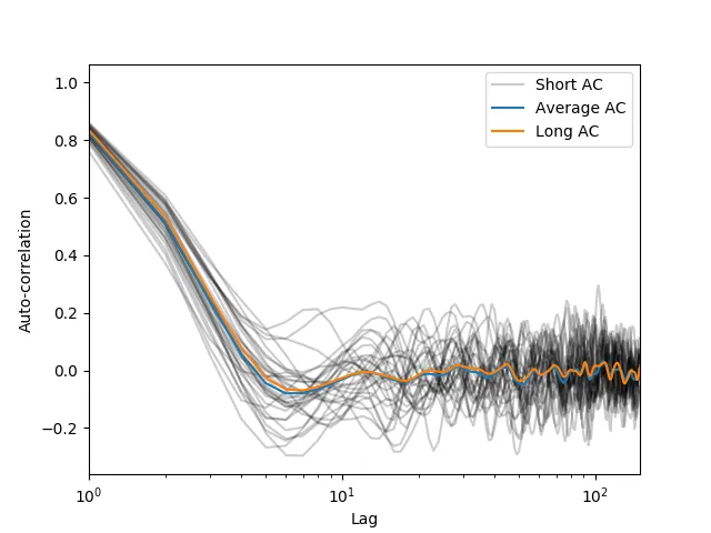
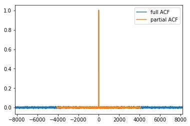
更新这是受@kazemakase回答启发的。我尝试用一些用于生成下面图像的代码来说明我的意思。可以看到@kazemakase是正确的，事实上AC函数自然地平均了噪声。然而，对于AC的平均处理具有更快的优势！np.correlate似乎缩放为缓慢的O(n^2)，而不是我希望通过使用FFT通过循环卷积计算相关性时期望的O(nlogn)...

from statsmodels.tsa.arima_model import ARIMA
import statsmodels as sm
import matplotlib.pyplot as plt
import numpy as np

np.random.seed(12345)
arparams = np.array([.75, -.25, 0.2, -0.15])
maparams = np.array([.65, .35])
ar = np.r_[1, -arparams] # add zero-lag and negate
ma = np.r_[1, maparams] # add zero-lag
x = sm.tsa.arima_process.arma_generate_sample(ar, ma, 10000)


def calc_rxx(x):
    x = x-x.mean()
    N = len(x)
    Rxx = np.correlate(x,x,mode="same")[N/2::]/N
    #Rxx = np.correlate(x,x,mode="same")[N/2::]/np.arange(N,N/2,-1)
    return  Rxx/x.var()

def avg_rxx(x,nperseg=1024):
    rxx_windows = []
    Nw = int(np.floor(len(x)/nperseg))
    print Nw
    first = True
    for i in range(Nw-1):
        xw = x[i*nperseg:nperseg*(i+1)]
        y = calc_rxx(xw)
        if i%1 == 0:
            if first:
                plt.semilogx(y,"k",alpha=0.2,label="Short AC")
                first = False
            else:
                plt.semilogx(y,"k",alpha=0.2)

        rxx_windows.append(y)
        
    print np.shape(rxx_windows)
    return np.mean(rxx_windows,axis=0)



plt.figure()
r_avg = avg_rxx(x,nperseg=300)
r = calc_rxx(x)
plt.semilogx(r_avg,label="Average AC")
plt.semilogx(r,label="Long AC")

plt.xlabel("Lag")
plt.ylabel("Auto-correlation")
plt.legend()
plt.xlim([0,150])
plt.show()

- Dipole

@CrazyIvan 抱歉我编辑了我的回答 - 我确实使用 same 选项。 - Dipole

你可能会在这个帖子中找到一些帮助：https://dev59.com/Z4vda4cB1Zd3GeqPca2x - Engineero

1个回答

网页内容由stack overflow 提供, 点击上面的

可以查看英文原文，
原文链接

- MB-F · Accepted Answer

TL-DR：为了减少自相关函数中的噪声，请增加信号x的长度。

分割数据并像频谱估计那样进行平均是一个有趣的想法。我希望它能够奏效...

自相关被定义为：

假设我们将数据分成两个窗口。它们的自相关性如下：

请注意，它们只在求和的限制上有所不同。基本上，我们将自相关的求和分为两部分。当我们将它们加起来时，我们回到了原始的自相关！所以我们没有获得任何东西。

结论是，在numpy/scipy中没有实现这样的东西，因为这样做没有意义。

备注：

我希望您能轻松看出这适用于任意数量的分区。
为了保持简单，我省略了归一化。如果你将 Rxx 除以 n 和部分 Rxx 除以 n/2，你会得到 Rxx / n == (Rxx1 * 2/n + Rxx2 * 2/n) / 2。也就是说，归一化部分自相关的平均值等于完整归一化自相关。
为了更简单，我假设信号 x 可以超出0和 n-1的限制进行索引。实际上，如果信号存储在数组中，这通常是不可能的。在这种情况下，完全自相关和部分自相关之间存在微小差异，随着滞后 l 的增加而增加。不幸的是，这只是一个精度损失，并不能减少噪音。

代码异端！我不相信你邪恶的数学！

当然，我们可以尝试一些东西并查看：

import matplotlib.pyplot as plt
import numpy as np

n = 2**16
n_segments = 8

x = np.random.randn(n)  # data

rx = np.correlate(x, x, mode='same') / n  # ACF
l1 = np.arange(-n//2, n//2)  # Lags

segments = x.reshape(n_segments, -1)
m = segments.shape[1]

rs = []
for y in segments:
    ry = np.correlate(y, y, mode='same') / m  # partial ACF
    rs.append(ry)

l2 = np.arange(-m//2, m//2)  # lags of partial ACFs

plt.plot(l1, rx, label='full ACF')
plt.plot(l2, np.mean(rs, axis=0), label='partial ACF')
plt.xlim(-m, m)
plt.legend()
plt.show()

尽管我们使用了8个段来平均自相关函数（ACF），但噪声水平在视觉上保持不变。

“好的，那么为什么它不起作用，但解决方案是什么？”

好消息是：自相关已经是一种降噪技术！至少在某种程度上是这样的：应用ACF的一个应用是查找被噪声隐藏的周期信号。

由于噪声（理想情况下）具有零均值，其影响会随着我们求和的元素数量增加而减小。换句话说，您可以通过使用更长的信号来减少自相关中的噪声。（我想这可能对于每种类型的噪声都不一定正确，但应该适用于通常的高斯白噪声及其相关类型。）

看吧，随着更多数据样本的出现，噪声变得更低了：

import matplotlib.pyplot as plt
import numpy as np

for n in [2**6, 2**8, 2**12]:
    x = np.random.randn(n)

    rx = np.correlate(x, x, mode='same') / n  # ACF
    l1 = np.arange(-n//2, n//2)  # Lags

    plt.plot(l1, rx, label='n={}'.format(n))

plt.legend()    
plt.xlim(-20, 20)
plt.show()