手动添加图例到ggplot2无效。

Question

手动添加图例到ggplot2无效。

3

我不仅搜索了stackoverflow，还查看了许多其他网站。不幸的是，我还没有找到任何帮助。我将尽可能明确地解释我的问题。由于这是我在stackoverflow上的第一个问题，所以请温柔些，我是R的完全初学者。我的目标是手动向已创建的ggplot2对象添加图例。

这是我正在使用的数据集：

structure(list(Values = 0:5, Count = c(213L, 128L, 37L, 18L, 
3L, 1L), rel_freq = c(0.5325, 0.32, 0.0925, 0.045, 0.0075, 0.0025
), pois_distr = c(0.505352031744286, 0.344902761665475, 0.117698067418343, 
0.0267763103376731, 0.00456870795136548, 0.000623628635361388
)), class = "data.frame", row.names = c(NA, -6L))

看起来像

  Values Count rel_freq   pois_distr
1      0   213   0.5325 0.5053520317
2      1   128   0.3200 0.3449027617
3      2    37   0.0925 0.1176980674
4      3    18   0.0450 0.0267763103
5      4     3   0.0075 0.0045687080
6      5     1   0.0025 0.0006236286

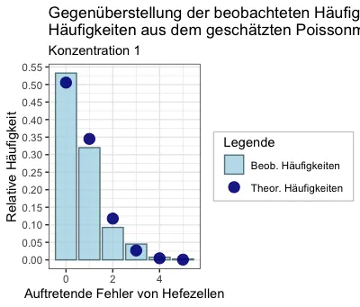
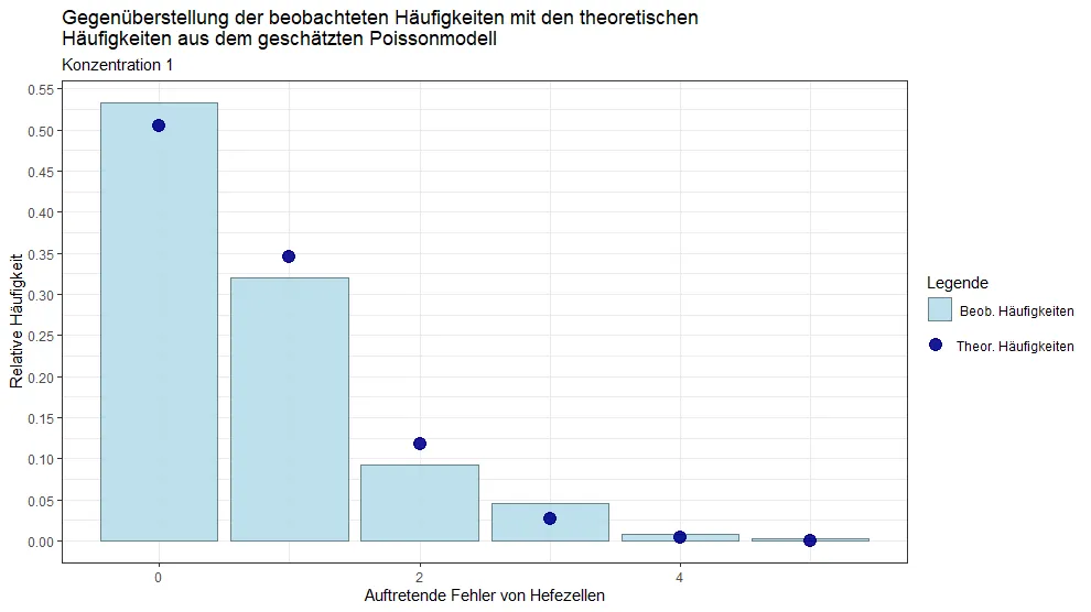
接下来，我已经成功创建了一个ggplot，它还不错，代码如下：

cols <- c('Beob. Häufigkeiten' = 'lightblue', 'Theor. Häufigkeiten' = 'darkblue')
plot_yeast1 <- ggplot(data.frame(data1_plot), aes(x=Values)) + 
  geom_col(aes(y=rel_freq, fill = 'Beob. Häufigkeiten'), col = 'lightblue4', alpha = 0.8) + 
  geom_point(aes(y=pois_distr, colour = 'Theor. Häufigkeiten'), alpha = 0.9, size = 4) +
  scale_fill_manual(name = 'Legende', values = cols) +
  scale_colour_manual(name ='Legende', values = cols) + 
  scale_y_continuous(breaks = seq(0, 0.6, 0.05)) +
  labs(title = 'Gegenüberstellung der beobachteten Häufigkeiten mit den theoretischen \nHäufigkeiten aus dem geschätzten Poissonmodell', x = 'Auftretende Fehler von Hefezellen', y = 'Relative Häufigkeit', subtitle = 'Konzentration 1') +
  theme_bw()
plot_yeast1

输出结果为：

同时显示两个标题的图表

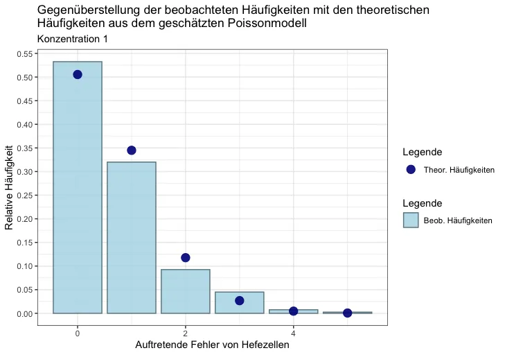
我的目标是将右侧手动创建的两个图例合并成一个。我已经尝试跳过第二个图例的标题，结果如下：

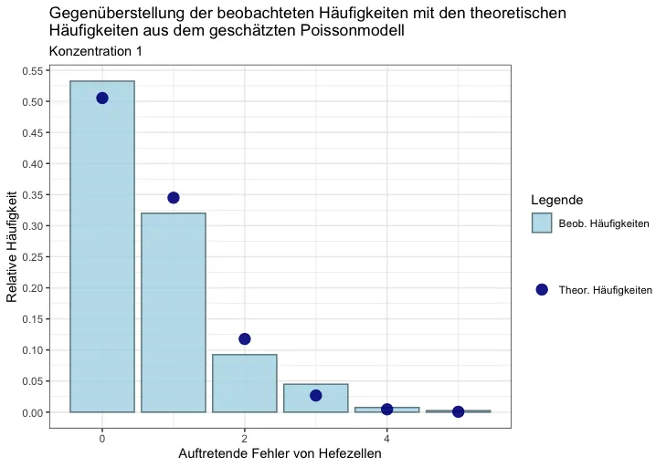
去掉第二个标题的图表。

但是这个空隙很丑陋，应该有一种方法将这两个图例合并成一个，在其中两个条目彼此接近。我已经花了超过9个小时来研究它，并查找了许多帖子，没有解决我的问题。如果有任何不清楚的地方，请告诉我。正如我已经写过的，这是第一次提出问题。谢谢

- m0byn

1

也与 https://dev59.com/26zka4cB1Zd3GeqP3h1M#50827425 相关的编程内容。请仅返回翻译后的文本。 - tjebo

2

顺便说一下，我有一些反馈：非常精心措辞的问题。感谢您以易于导入和处理的格式提供详细信息、代码和数据。这些细节非常受欢迎，并且肯定会为您获得可用答案提供最好的机会！ - chemdork123

2个回答

2

您可以使用 theme(legend.margin) 将图例紧凑排列，如下所示。

cols <- c('Beob. Häufigkeiten' = 'lightblue', 'Theor. Häufigkeiten' = 'darkblue')
plot_yeast1 <- ggplot(data.frame(data1_plot), aes(x=Values)) + 
  geom_col(aes(y=rel_freq, fill = 'Beob. Häufigkeiten'), col = 'lightblue4', alpha = 0.8) + 
  geom_point(aes(y=pois_distr, colour = 'Theor. Häufigkeiten'), alpha = 0.9, size = 4) +
  scale_fill_manual(name = 'Legende', values = cols) +
  scale_colour_manual(name =NULL, values = cols) + 
  scale_y_continuous(breaks = seq(0, 0.6, 0.05)) +
  labs(title = 'Gegenüberstellung der beobachteten Häufigkeiten mit den theoretischen \nHäufigkeiten aus dem geschätzten Poissonmodell', x = 'Auftretende Fehler von Hefezellen', y = 'Relative Häufigkeit', subtitle = 'Konzentration 1') +
  theme_bw() +
  theme(
    # legend.position = c(.95, .95),
    # legend.justification = c("right", "top"),
    legend.box.just = "right",
    legend.margin = margin(-10)
  )
plot_yeast1

- Greg

非常感谢！ - m0byn

网页内容由stack overflow 提供, 点击上面的

可以查看英文原文，
原文链接

- Wolfgang Arnold · Accepted Answer

如果主要是通过视觉方式将两个传说组合成一个，那么这种方法可能会有所帮助 - 详见在末尾处调用theme(...)的注释。

cols <- c('Beob. Häufigkeiten' = 'lightblue', 'Theor. Häufigkeiten' = 'darkblue')
plot_yeast1 <- ggplot(data.frame(data1_plot), aes(x=Values)) + 
  geom_col(aes(y=rel_freq, fill = 'Beob. Häufigkeiten'), col = 'lightblue4', alpha = 0.8) + 
  geom_point(aes(y=pois_distr, colour = 'Theor. Häufigkeiten'), alpha = 0.9, size = 4) +
  scale_fill_manual(name = 'Legende', values = cols) +
  scale_colour_manual(name ='', values = cols) + 
  scale_y_continuous(breaks = seq(0, 0.6, 0.05)) +
  labs(title = 'Gegenüberstellung der beobachteten Häufigkeiten mit den theoretischen \nHäufigkeiten aus dem geschätzten Poissonmodell', x = 'Auftretende Fehler von Hefezellen', y = 'Relative Häufigkeit', subtitle = 'Konzentration 1') +
  theme_bw() +
  theme(legend.box.background = element_rect(colour = "grey", fill = "white"), # create a box around all legends
        legend.box.margin = margin(0.1, 0.1, 0.1, 0.1, "cm"),                  # specify the margin of that box
        legend.background = element_blank(),                                   # remove boxes around legends (redundant here, as theme_bw() seems to do that already)
        legend.spacing = unit(-0.5, "cm"),                                     # move legends closer together
        legend.margin = margin(0, 0.2, 0, 0.2, "cm"))                          # specify margins of each legend: top and bottom 0 to move them closer
plot_yeast1