我不确定如何做这件事,但是我收到了一个例子,例如频谱图,但是这是一个二维的图像。
我有一段代码生成了混合频率,并且在fft中可以选择这些频率,但是我该如何在频谱图中看到这些频率?我知道我的例子中频率并没有随时间变化,那么这是否意味着我会在频谱图上看到一条直线?
以下是我的代码和输出图片:
我有一段代码生成了混合频率,并且在fft中可以选择这些频率,但是我该如何在频谱图中看到这些频率?我知道我的例子中频率并没有随时间变化,那么这是否意味着我会在频谱图上看到一条直线?
以下是我的代码和输出图片:
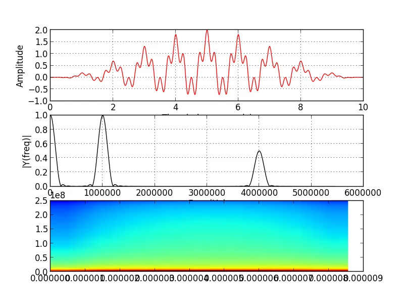
# create a wave with 1Mhz and 0.5Mhz frequencies
dt = 2e-9
t = np.arange(0, 10e-6, dt)
y = np.cos(2 * pi * 1e6 * t) + (np.cos(2 * pi * 2e6 *t) * np.cos(2 * pi * 2e6 * t))
y *= np.hanning(len(y))
yy = np.concatenate((y, ([0] * 10 * len(y))))
# FFT of this
Fs = 1 / dt # sampling rate, Fs = 500MHz = 1/2ns
n = len(yy) # length of the signal
k = np.arange(n)
T = n / Fs
frq = k / T # two sides frequency range
frq = frq[range(n / 2)] # one side frequency range
Y = fft(yy) / n # fft computing and normalization
Y = Y[range(n / 2)] / max(Y[range(n / 2)])
# plotting the data
subplot(3, 1, 1)
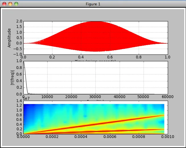
plot(t * 1e3, y, 'r')
xlabel('Time (micro seconds)')
ylabel('Amplitude')
grid()
# plotting the spectrum
subplot(3, 1, 2)
plot(frq[0:600], abs(Y[0:600]), 'k')
xlabel('Freq (Hz)')
ylabel('|Y(freq)|')
grid()
# plotting the specgram
subplot(3, 1, 3)
Pxx, freqs, bins, im = specgram(y, NFFT=512, Fs=Fs, noverlap=10)
show()
import语句。 - wizzwizz4