ggplot2：如何将坐标轴标题放在图表区域内

Question

ggplot2：如何将坐标轴标题放在图表区域内

3

我想创建一个ggplot2图，其中y轴和x轴标签都在内部，即朝内并放置在绘图区域内。

这个之前的SO答案由Z.Lin解决了y轴的情况，我已经成功地实现了。但是将该方法扩展到两个轴让我感到困惑。grobs很难处理，我认为。

所以我试图从小处开始，通过改编Z.Lin的代码使其适用于x轴而不是y轴，但我甚至没有能够实现这一点。grobs真的很复杂。我的尝试（如下）在没有错误/警告的情况下运行，直到grid.draw()，那里它就会崩溃（我认为我在某个地方误用了一些参数，但我无法确定哪个，在这一点上我只是在猜测）。

# locate the grob that corresponds to x-axis labels
x.label.grob <- gp$grobs[[which(gp$layout$name == "axis-b")]]$children$axis

# remove x-axis labels from the plot, & shrink the space occupied by them
gp$grobs[[which(gp$layout$name == "axis-b")]] <- zeroGrob()
gp$widths[gp$layout$l[which(gp$layout$name == "axis-b")]] <- unit(0, "cm")

# create new gtable
new.x.label.grob <- gtable::gtable(widths = unit(1, "npc"))
# place axis ticks in the first row
new.x.label.grob <- 
   gtable::gtable_add_rows(
      new.x.label.grob,
      heights = x.label.grob[["heights"]][1])
new.x.label.grob <- 
   gtable::gtable_add_grob(
      new.x.label.grob,
      x.label.grob[["grobs"]][[1]],
      t = 1, l = 1)
# place axis labels in the second row
new.x.label.grob <- 
   gtable::gtable_add_rows(
      new.x.label.grob,
      heights = x.label.grob[["heights"]][2])
new.x.label.grob <- 
   gtable::gtable_add_grob(
      new.x.label.grob,
      x.label.grob[["grobs"]][[2]],
      t = 1, l = 2)
# add third row that takes up all the remaining space
new.x.label.grob <- 
   gtable::gtable_add_rows(
      new.x.label.grob,
      heights = unit(1, "null"))

gp <- 
   gtable::gtable_add_grob(
      x = gp,
      grobs = new.x.label.grob,
      t = gp$layout$t[which(gp$layout$name == "panel")],
      l = gp$layout$l[which(gp$layout$name == "panel")])
grid.draw(gp)
# Error in unit(widths, default.units) : 
#  'x' and 'units' must have length > 0

我想我的问题可以分成三个半独立的部分，每个后续问题都取代了之前的问题（因此，如果您可以回答较晚的问题，就不需要打扰之前的问题）：

有人能够将现有答案适应于x轴吗？
有人能够提供相应的代码来使两个轴内部显示吗？
有人知道更简洁的方法来实现ggplot2中的两个轴内部显示吗？

这是我的MWE（大部分是复制了Z.Lin的答案，但使用了新数据）：

library(dplyr)
library(magrittr)
library(ggplot2)
library(grid)
library(gtable)
library(errors)
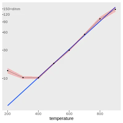
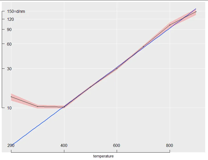
df <- structure(list(
   temperature = c(200, 300, 400, 500, 600, 700, 800, 900), 
   diameter = 
      structure(
         c(13.54317, 10.32521, 10.23137, 17.90464, 29.98183, 55.65514, 101.60747, 147.3074), 
         id = "<environment>", 
         errors = c(1.24849, 0.46666, 0.36781, 0.48463, 0.94639, 1.61459, 6.98346, 12.18353), 
         class = "errors")), 
   row.names = c(NA, -8L), 
   class = "data.frame")
p <- ggplot() +
   geom_smooth(data = df %>% filter(temperature >= 400),
               aes(x = temperature, y = diameter),
               method = "lm", formula = "y ~ x",
               se = FALSE, fullrange = TRUE) +
   # experimental errors as red ribbon (instead of errorbars)
   geom_ribbon(data = df,
               aes(x = temperature, 
                   ymin = errors_min(diameter), 
                   ymax = errors_max(diameter)), 
               fill = alpha("red", 0.2),
               colour = alpha("red", 0.2)) +
   geom_point(data = df,
              aes(x = temperature, y = diameter),
              size = 0.7) +
   geom_line(data = df,
             aes(x = temperature, y = diameter),
             size = 0.15) +
   scale_x_continuous(breaks = seq(200, 900, 200)) +
   scale_y_log10(breaks = c(10, seq(30, 150, 30)),
                 labels = c("10", "30", "60", "90", "120", "150=d/nm")) +
   theme(panel.grid.major = element_blank(), 
         panel.grid.minor = element_blank(), 
         axis.title.y = element_blank(),
         axis.text.y = element_text(hjust = 0))
# convert from ggplot to grob object
gp <- ggplotGrob(p)
y.label.grob <- gp$grobs[[which(gp$layout$name == "axis-l")]]$children$axis
gp$grobs[[which(gp$layout$name == "axis-l")]] <- zeroGrob()
gp$widths[gp$layout$l[which(gp$layout$name == "axis-l")]] <- unit(0, "cm")
new.y.label.grob <- gtable::gtable(heights = unit(1, "npc"))
new.y.label.grob <- 
   gtable::gtable_add_cols(
      new.y.label.grob,
      widths = y.label.grob[["widths"]][2])
new.y.label.grob <- 
   gtable::gtable_add_grob(
      new.y.label.grob,
      y.label.grob[["grobs"]][[2]],
      t = 1, l = 1)
new.y.label.grob <- 
   gtable::gtable_add_cols(
      new.y.label.grob,
      widths = y.label.grob[["widths"]][1])
new.y.label.grob <- 
   gtable::gtable_add_grob(
      new.y.label.grob,
      y.label.grob[["grobs"]][[1]],
      t = 1, l = 2)
new.y.label.grob <- 
   gtable::gtable_add_cols(
      new.y.label.grob,                                    
      widths = unit(1, "null"))
gp <- 
   gtable::gtable_add_grob(
      x = gp,
      grobs = new.y.label.grob,
      t = gp$layout$t[which(gp$layout$name == "panel")],
      l = gp$layout$l[which(gp$layout$name == "panel")])
grid.draw(gp)

> sessionInfo()
R version 3.6.2 (2019-12-12)
Platform: x86_64-pc-linux-gnu (64-bit)
Running under: Ubuntu 18.04.5 LTS

Matrix products: default
BLAS:   /usr/lib/x86_64-linux-gnu/blas/libblas.so.3.7.1
LAPACK: /usr/lib/x86_64-linux-gnu/lapack/liblapack.so.3.7.1

locale:
 [1] LC_CTYPE=en_GB.UTF-8       LC_NUMERIC=C              
 [3] LC_TIME=en_GB.UTF-8        LC_COLLATE=en_GB.UTF-8    
 [5] LC_MONETARY=en_GB.UTF-8    LC_MESSAGES=en_GB.UTF-8   
 [7] LC_PAPER=en_GB.UTF-8       LC_NAME=C                 
 [9] LC_ADDRESS=C               LC_TELEPHONE=C            
[11] LC_MEASUREMENT=en_GB.UTF-8 LC_IDENTIFICATION=C       

attached base packages:
[1] grid      stats     graphics  grDevices utils     datasets  methods  
[8] base     

other attached packages:
[1] errors_0.3.4  gtable_0.3.0  ggplot2_3.3.2 magrittr_1.5  dplyr_1.0.2  

loaded via a namespace (and not attached):
 [1] rstudioapi_0.11  splines_3.6.2    tidyselect_1.1.0 munsell_0.5.0   
 [5] lattice_0.20-41  colorspace_1.4-1 R6_2.5.0         rlang_0.4.8     
 [9] tools_3.6.2      nlme_3.1-148     mgcv_1.8-31      withr_2.3.0     
[13] ellipsis_0.3.1   digest_0.6.27    yaml_2.2.1       tibble_3.0.4    
[17] lifecycle_0.2.0  crayon_1.3.4     Matrix_1.2-18    purrr_0.3.4     
[21] farver_2.0.3     vctrs_0.3.4      glue_1.4.2       compiler_3.6.2  
[25] pillar_1.4.6     generics_0.1.0   scales_1.1.1     pkgconfig_2.0.3

- solarchemist

2个回答

2

如果有人正在寻找使用ggplot2制作紧凑型图形的方法，例如用于放置在页面边距内，那么您可能会通过上面答案中Allan Cameron优雅的方法提供的完整代码获得帮助。

将图形放置在页面边距内通常不可取，并且取决于可用的边距、文档类型等。无论如何，最好尽可能使图形简洁流畅。这就是为什么在我的情况下，我正在寻找一种方式来保持尽可能多的图形位于面板的占地面积内。

足够的背景知识，以下是代码：

library(dplyr)
library(magrittr)
library(ggplot2)
library(grid)
library(gtable)
library(errors)
theme_set(theme_grey())

move_axes_inside <- function(p) {
   b <- ggplot_build(p)
   x_breaks <- b$layout$panel_scales_x[[1]]$break_info()
   y_breaks <- b$layout$panel_scales_y[[1]]$break_info()
   x_range <- b$layout$panel_params[[1]]$x.range
   y_range <- b$layout$panel_params[[1]]$y.range
   y_breaks$major <- 
      diff(y_breaks$range) / diff(y_range) * y_breaks$major + 
      (y_breaks$range[1] - y_range[1]) / diff(y_range)
   x_breaks$major <- 
      diff(x_breaks$range) / diff(x_range) * x_breaks$major + 
      (x_breaks$range[1] - x_range[1]) / diff(x_range)
   y <- 
      grid::yaxisGrob(
         at = y_breaks$major, 
         label = y_breaks$labels, 
         gp = 
            gpar(
               lwd = 1, # line width of axis and tick marks
               fontsize = 8,
               cex = 0.8, # multiplier to font size
               lineheight = 0.8), # tick mark length
         main = FALSE)
   x <- 
      grid::xaxisGrob(
         at = x_breaks$major, 
         label = x_breaks$labels, 
         gp = 
            gpar(
               lwd = 2, # draw axis with thicker line width
               fontsize = 8,
               cex = 0.8, # multiplier to font size
               lineheight = 0.8), # tick mark length
         main = FALSE)
   p <- 
      p + 
      annotation_custom(
         # draw y-axis, shifted slightly inwards (so that axis is inside panel.border)
         grob = y, 
         xmin = x_range[1] + 0.01 * diff(x_range), 
         xmax = x_range[1] + 0.01 * diff(x_range)) +
      annotation_custom(
         grob = x, 
         ymin = y_range[1] + 0.01 * diff(y_range),
         ymax = y_range[1] + 0.01 * diff(y_range)) +
      theme(
         axis.ticks = element_blank(),
         axis.title.y = element_blank(),
         axis.text.y = element_blank(),
         axis.text.x = element_blank())
   return(p)
}

p <- ggplot() +
   geom_line(
      stat = "smooth", method = lm, formula = "y ~ x",
      se = FALSE, fullrange = TRUE,
      data = df %>% filter(temperature >= 400),
      aes(x = temperature, y = diameter),
      colour = "blue", size = 2, alpha = 0.35) +
   # experimental errors as red ribbon (instead of errorbars)
   geom_ribbon(
      data = df,
      aes(x = temperature, 
          ymin = errors_min(diameter), 
          ymax = errors_max(diameter)), 
      fill = alpha("red", 0.25),
      colour = NA) +
   # data points excluded in linear fit
   geom_point(
      data = df %>% filter(temperature < 400),
      aes(x = temperature, y = diameter),
      # by default, shape=19 (filled circle)
      # https://blog.albertkuo.me/post/point-shape-options-in-ggplot/
      # I'd like a solid circle, so shape 16 it is
      size = 1.2, shape = 16, colour = alpha("red", 0.25)) +
   # data points included in linear fit
   geom_point(
      data = df %>% filter(temperature >= 400),
      aes(x = temperature, y = diameter),
      size = 1.2, shape = 16, colour = alpha("red", 0.45)) +
   # I ended up putting the x-axis unit label on the outside because 
   # however I tried, it would not fit inside and I was not able to 
   # rotate the x-axis labels on the inside.
   labs(x = "$T_\\mathrm{a}/\\si{\\celsius}$") +
   scale_x_continuous(
      breaks = seq(200, 900, 100),
      # first element can't be empty string - if so then all labels dont print (weird bug?)
      labels = c(" ", " ", "400", " ", "600", " ", "800", " ")) +
   scale_y_log10(
      breaks = c(10, 50, 90, 130),
      labels = c("\\num{10}", "\\num{50}", "\\num{90}", "$\\num{130}=d/\\si{\\nm}$")) +
   # note that we set some theme settings inside the move_axes_inside() function
   theme(
      # l = -1 was required to completely fill the space with plot panel
      # b = 0 because we are making room for x-axis title on the outside
      plot.margin = margin(t = 0, r = 0, b = 0, l = -1, "mm"),
      # smaller text size in x-axis title, trying to conform with fontsize inside axis
      # vjust moves the title closer to the x-axis line, value optimised optically
      axis.title.x = element_text(size = 8 * 0.8, vjust = 2.0),
      # grid lines just look busy in such a small plot
      panel.grid.major = element_blank(),
      panel.grid.minor = element_blank())

move_axes_inside(p)

这是一张屏幕截图，位于使用knitr和LaTeX编译的文档中，并且将绘图放在\marginpar{}中：

- solarchemist

网页内容由stack overflow 提供, 点击上面的

可以查看英文原文，
原文链接

- Allan Cameron · Accepted Answer

与其将图形冻结为 grob 树，然后对 grobs 进行操作，不如尝试将坐标轴移动到内部但保持对象为 ggplot，这样会更有用。实现方法是编写一个函数，该函数接受您的图形，提取必要信息，然后构建轴并将它们作为注释添加。

返回的对象是一个普通的 ggplot，您可以像平常一样添加图层、比例和修改主题。

move_axes_inside <- function(p)
{
  b <- ggplot_build(p)
  x_breaks <- b$layout$panel_scales_x[[1]]$break_info()
  y_breaks <- b$layout$panel_scales_y[[1]]$break_info()
  x_range <- b$layout$panel_params[[1]]$x.range
  y_range <- b$layout$panel_params[[1]]$y.range
  y_breaks$major <- diff(y_breaks$range)/diff(y_range) * y_breaks$major + 
    (y_breaks$range[1] - y_range[1])/diff(y_range)
  x_breaks$major <- diff(x_breaks$range)/diff(x_range) * x_breaks$major + 
    (x_breaks$range[1] - x_range[1])/diff(x_range)
  y <- grid::yaxisGrob(at = y_breaks$major, label = y_breaks$labels, main = FALSE)
  x <- grid::xaxisGrob(at = x_breaks$major, label = x_breaks$labels, main = FALSE)
  p + annotation_custom(y, xmin = x_range[1], xmax = x_range[1]) +
      annotation_custom(x, ymin = y_range[1], ymax = y_range[1]) +
      theme(axis.text.y = element_blank(),
            axis.ticks = element_blank(),
            axis.text.x = element_blank())
    
}

使用您的情节进行测试，我们得到：

p2 <- move_axes_inside(p)
 
p2

我们可以更改主题元素等。

p2 + theme(panel.grid.major = element_line())

这需要一些开发和测试才能让它适用于离散轴等情况，但它应该可以直接用于任意连续轴。