如何在Python中解释离散傅里叶变换（FFT）的结果

Question

这个主题有很多问题，我已经浏览了很多，获取了处理频率的概念指针（这里和这里），numpy函数的文档（这里），提取幅度和相位的操作信息（这里），以及在站外查找，例如这个或这个。

然而，只有通过简单的例子证明并检查不同函数的输出与其手动实现相对比，才给我留下了一点想法。

答案试图记录并分享有关Python中DFT的细节，如果不用简单的术语解释可能会构成入门障碍。

- Antoni Parellada

Answer 1

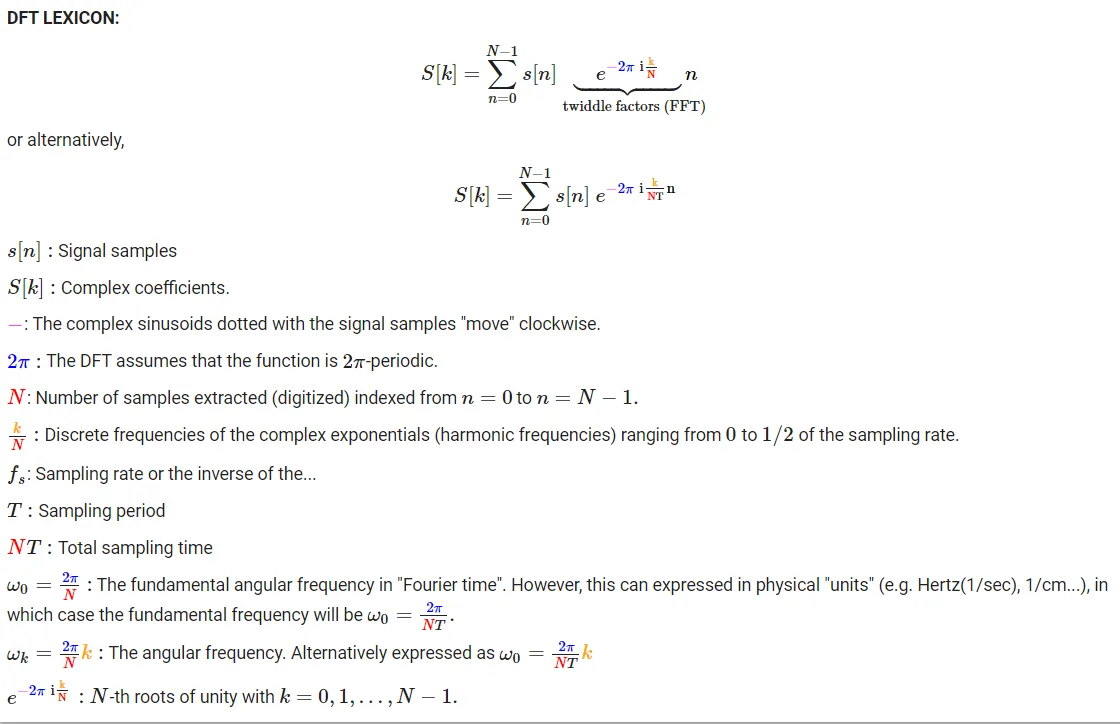
DFT（FFT是其算法计算）是模拟信号s（时间或空间函数）的有限离散样本N与一组复指数基向量（正弦和余弦函数）之间的点积。尽管样本自然是有限的，可能没有周期性，但它被隐式地认为是一个周期性重复的离散函数。即使处理实值信号（通常情况下），使用复数（欧拉方程）也很方便。在使用np.fft.fft(s)对信号进行函数实现时，只能获得复数输出系数并陷入它们的解释中，这可能令人望而生畏。有些步骤是必不可少的：

复指数中的频率是什么？

1. DFT不一定保留赫兹的采样频率。频率是指标号（k）。
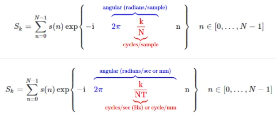
2. 标号k的范围为0到N-1，可以看作是具有单位cycles / set的量（其中set是信号s的N个样本）。我将省略讨论奈奎斯特极限，但对于实际信号，频率在N/2之后形成镜像，并在该点之后以负递减值给出（在隐含周期性的框架内不是问题）。FFT中使用的频率不仅仅是k，而是k/N，被认为具有cycles / sample的单位。请参见this reference。示例（reference）：如果一个信号被采样了N=5次，则频率为：np.fft.fftfreq(5)，得到[0,0.2,0.4,-0.4,-0.2]，即[0/5,1/5,2/5,-2/5,-1/5]。
3. 要将这些频率转换为有意义的单位（例如Hetz或mm），需要将上面的cycles/sample值除以采样间隔T（例如样本之间的秒数距离）。继续上面的例子，有一个内置调用：np.fft.fftfreq(5, d=T)：如果模拟信号s在等距间隔T=1/2秒内采样了5次，总共采样了NT=5 x 1/2 sec，则标准化频率将为np.fft.fftfreq(5, d = 1/2)，得到[0 0.4 0.8 -0.8 -0.4]或[0/NT, 1/NT, 2/NT, -2/NT, -1/NT]。
4. 规范化或未规范化的频率都用于控制角频率（ω_m），表示为ω_m=2πk/NT。请注意，NT是信号被采样的总持续时间。索引k确实会产生基本频率（ω-naught）的倍数，对应于完成在NT上恰好一次振荡的（余）正弦波的频率（here）。

FFT中系数的幅度、频率和相位

1. 给定FFT的输出S = fft.fft(s)，输出系数的幅度（此处）只是调整为实信号对称性和样本数量1/N后的复杂数的欧几里得范数：magnitudes = 1/N * np.abs(S)
2. 频率与上述调用匹配np.fft.fftfreq(N)，或更方便地将实际模拟频率单位合并：frequencies = np.fft.fftfreq(N, d=T)。
3. 每个系数的相位是极坐标形式中的复数角度：phase = np.arctan(np.imag(S)/np.real(S))

---

如何在FFT中找到信号s中的主频率及其系数？

1. 除了绘图，可以通过以下方法找到幅度最高的频率对应的索引k： index = np.argmax(np.abs(S))。例如，要找到具有最高幅度的4个索引，则调用为indices = np.argpartition(S,-4)[-4:]。
2. 并找到实际对应的系数：S[index]与频率freq_max = np.fft.fftfreq(N, d=T)[index]。

---

获得系数后重现原始信号：

通过正弦和余弦函数重现s（参见此处的第150页）：

    Re = np.real(S[index])
    Im = np.imag(S[index])
    
    s_recon = Re * 2/N * np.cos(-2 * np.pi * freq_max * t) + abs(Im) * 2/N * np.sin(-2 * np.pi * freq_max * t) 

这是一个完整的例子：

import numpy as np
import matplotlib.pyplot as plt

N = 10000           # Sample points     
T = 1/5000          # Spacing
# Total duration N * T= 2
t = np.linspace(0.0, N*T, N, endpoint=False) # Time: Vector of 10,000 elements from 0 to N*T=2.
frequency = np.fft.fftfreq(t.size, d=T)      # Normalized Fourier frequencies in spectrum.

f0 = 25             # Frequency of the sampled wave
phi = np.pi/8       # Phase
A = 50              # Amplitude

s = A * np.cos(2 * np.pi * f0 * t + phi) # Signal

S = np.fft.fft(s)   # Unnormalized FFT

index = np.argmax(np.abs(S))
print(S[index])
magnitude = np.abs(S[index]) * 2/N
freq_max = frequency[index]

phase = np.arctan(np.imag(S[index])/np.real(S[index]))
print(f"magnitude: {magnitude}, freq_max: {freq_max}, phase: {phase}")
print(phi)

fig, [ax1,ax2] = plt.subplots(nrows=2, ncols=1, figsize=(10, 5))
ax1.plot(t,s, linewidth=0.5, linestyle='-', color='r', marker='o', markersize=1,markerfacecolor=(1, 0, 0, 0.1))  
ax1.set_xlim([0, .31])
ax1.set_ylim([-51,51])
ax2.plot(frequency[0:N//2], 2/N * np.abs(S[0:N//2]), '.', color='xkcd:lightish blue', label='amplitude spectrum')
plt.xlim([0, 100])
plt.show()

Re = np.real(S[index])
Im = np.imag(S[index])

s_recon = Re*2/N * np.cos(-2 * np.pi * freq_max * t) + abs(Im)*2/N * np.sin(-2 * np.pi * freq_max * t)

fig = plt.figure(figsize=(10, 2.5))

plt.xlim(0,0.3)
plt.ylim(-51,51)
plt.plot(t,s_recon, linewidth=0.5, linestyle='-', color='r', marker='o', markersize=1,markerfacecolor=(1, 0, 0, 0.1))  
plt.show()

s.all() == s_recon.all()

- Antoni Parellada