在MATLAB中为FFT缩放振幅两倍

Question

在MATLAB中为FFT缩放振幅两倍

3

我刚刚阅读了Matlab教程的示例，试图学习FFT函数。有人能告诉我为什么在最后一步中P1(2:end-1) = 2*P1(2:end-1)。在我看来，没有必要乘以2。

Fs = 1000;            % Sampling frequency
T = 1/Fs;             % Sampling period
L = 1000;             % Length of signal
t = (0:L-1)*T;        % Time vector

%--------
S = 0.7*sin(2*pi*50*t) + sin(2*pi*120*t);
%---------
X = S + 2*randn(size(t));
%---------
plot(1000*t(1:50),X(1:50))
title('Signal Corrupted with Zero-Mean Random Noise')
xlabel('t (milliseconds)')
ylabel('X(t)')

Y = fft(X);
P2 = abs(Y/L);
P1 = P2(1:L/2+1);
P1(2:end-1) = 2*P1(2:end-1);
f = Fs*(0:(L/2))/L;
plot(f,P1)
title('Single-Sided Amplitude Spectrum of X(t)')
xlabel('f (Hz)')
ylabel('|P1(f)|')

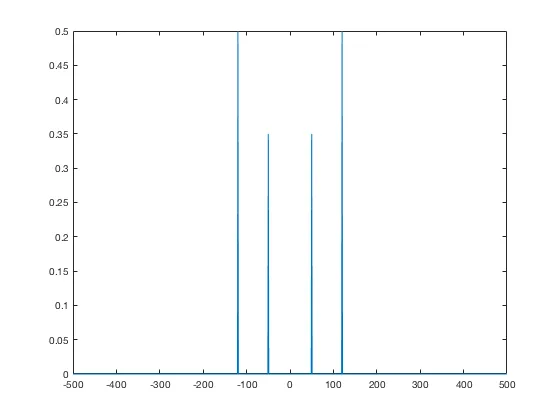
Y = fft(S);
P2 = abs(Y/L);
P1 = P2(1:L/2+1);
P1(2:end-1) = 2*P1(2:end-1);

plot(f,P1)
title('Single-Sided Amplitude Spectrum of S(t)')
xlabel('f (Hz)')
ylabel('|P1(f)|')

Matlab示例

- DaMi

1个回答

网页内容由stack overflow 提供, 点击上面的

可以查看英文原文，
原文链接

- Suever · Accepted Answer

乘以2的原因是由于fft返回的频谱关于直流分量对称。由于他们显示的是单面幅度谱，每个点的幅度将会加倍，以考虑频谱的另一侧的数据贡献。例如，pi/4的单面幅度是pi/4处的幅度加上-pi/4处的幅度。

第一个样本被跳过，因为它是直流点，因此在频谱的两侧共享。

因此，例如，如果我们查看其示例信号的fft，其中包含幅度为0.7的50Hz正弦波和幅度为1的120Hz正弦波。

Fs = 1000;            % Sampling frequency
T = 1/Fs;             % Sampling period
L = 1000;             % Length of signal
t = (0:L-1)*T;        % Time vector

S = 0.7*sin(2*pi*50*t) + sin(2*pi*120*t);

% Compute the FFT
Y = fft(S);

% Compute the amplitudes
amplitude = abs(Y / L);

% Figure out the corresponding frequencies
f = Fs/L*[0:(L/2-1),-L/2:-1]

% Plot the result
plot(f, amplitude)

当我们绘制它时，您会发现它是对称的，并且只有通过组合频谱两侧的振幅才能实现原始输入振幅。

他们所做的稍微更明确的版本是以下内容，它将频谱的两半部分相加。

P1(2:end-1) = P1(2:end-1) + P2((L/2+2):end);

但是由于光谱在定义上是对称的，所以可以选择简单地乘以2。