R平滑样条函数smooth.spline()：平滑样条不光滑反而过度拟合我的数据。

Question

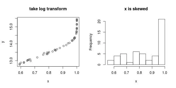
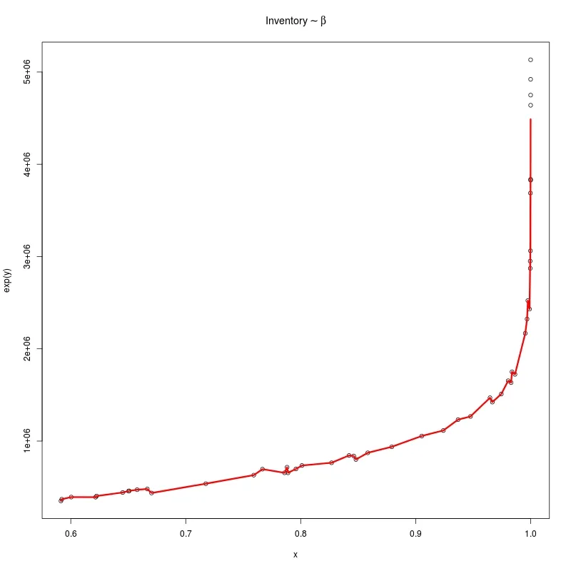
我有几个数据点，似乎适合通过它们拟合样条曲线。但是当我这样做时，我得到了一个相当崎岖的拟合，就像过度拟合一样，这不是我理解的平滑处理。

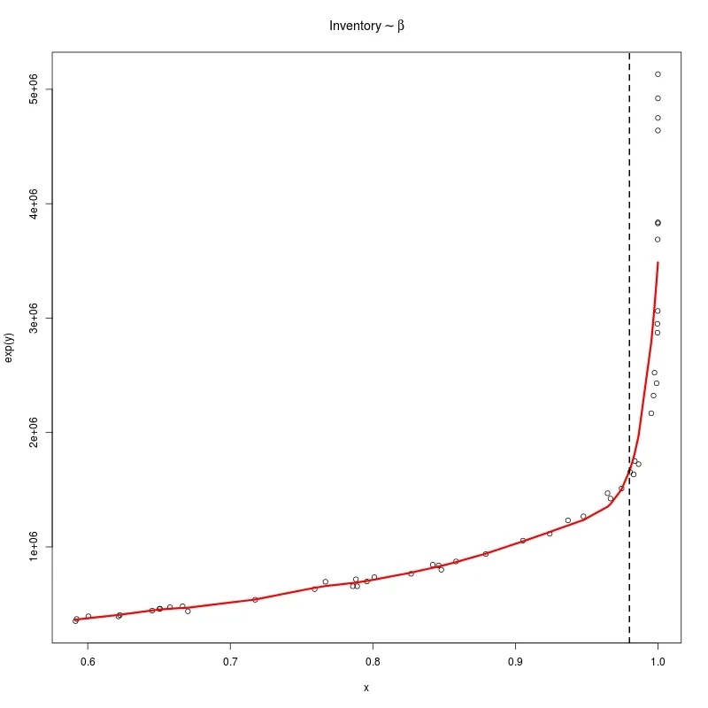
是否有特殊选项/参数可以获得真正平滑的样条曲线函数呢？ 像此处一样。

对于smooth.spline 的penalty 参数的使用似乎没有任何可见影响。也许我做错了吗？

以下是数据和代码：

results <- structure(
    list(
        beta = c(
            0.983790622281964, 0.645152464354322,
            0.924104713597375, 0.657703886566088, 0.788138034115623, 0.801080207252363,
            1, 0.858337365965949, 0.999687052533693, 0.666552625121279, 0.717453633245958,
            0.621570152961453, 0.964658181346544, 0.65071758770312, 0.788971505000918,
            0.980476054183113, 0.670263506919246, 0.600387040967624, 0.759173403408052,
            1, 0.986409675965, 0.982996471134736, 1, 0.995340781899163, 0.999855895958986,
            1, 0.846179233381267, 0.879226324448832, 0.795820998892035, 0.997586607285667,
            0.848036806290156, 0.905320944437968, 0.947709125535428, 0.592172373022407,
            0.826847031044922, 0.996916006944244, 0.785967729206612, 0.650346929853076,
            0.84206351833549, 0.999043126652724, 0.936879214753098, 0.76674066557003,
            0.591431233516217, 1, 0.999833445117791, 0.999606223666537, 0.6224971799303,
            1, 0.974537160571494, 0.966717133936379
        ), inventoryCost = c(
            1750702.95138889,
            442784.114583333, 1114717.44791667, 472669.357638889, 716895.920138889,
            735396.180555556, 3837320.74652778, 872873.4375, 2872414.93055556,
            481095.138888889, 538125.520833333, 392199.045138889, 1469500.95486111,
            459873.784722222, 656220.486111111, 1654143.83680556, 437511.458333333,
            393295.659722222, 630952.170138889, 4920958.85416667, 1723517.10069444,
            1633579.86111111, 4639909.89583333, 2167748.35069444, 3062420.65972222,
            5132702.34375, 838441.145833333, 937659.288194444, 697767.1875,
            2523016.31944444, 800903.819444444, 1054991.49305556, 1266970.92013889,
            369537.673611111, 764995.399305556, 2322879.6875, 656021.701388889,
            458403.038194444, 844133.420138889, 2430700, 1232256.68402778,
            695574.479166667, 351348.524305556, 3827440.71180556, 3687610.41666667,
            2950652.51736111, 404550.78125, 4749901.64930556, 1510481.59722222,
            1422708.07291667
        )
    ), .Names = c("beta", "inventoryCost"), class = c("data.frame")
)

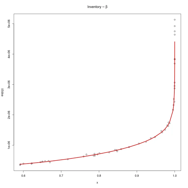
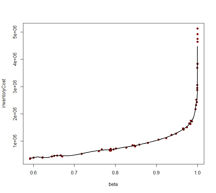
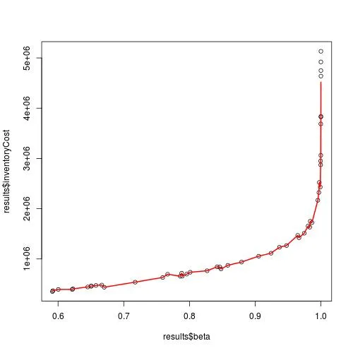
plot(results$beta,results$inventoryCost)
mySpline <- smooth.spline(results$beta,results$inventoryCost, penalty=999999)
lines(mySpline$x, mySpline$y, col="red", lwd = 2)

- mondano

Answer 1

在建模之前，合理地转换数据

基于你的results$inventoryCost的数值范围，对数变换是合适的。为了方便起见，在接下来的步骤中我将使用x、y进行表示，并重新排列数据使得x按升序排列：

x <- results$beta; y <- log(results$inventoryCost)
reorder <- order(x); x <- x[reorder]; y <- y[reorder]

par(mfrow = c(1,2))
plot(x, y, main = "take log transform")
hist(x, main = "x is skewed")

左边的图看起来更好吗？此外，强烈建议对 x 进行进一步的转换，因为它是倾斜的！（见右图）。

适当的变换如下：

x1 <- -(1-x)^(1/3)

立方根(1-x)将使数据在x = 1周围更加分散。 我添加了-1以确保x和x1之间存在正单调关系，而不是负单调关系。 现在让我们来检查这种关系：

par(mfrow = c(1,2))
plot(x1, y, main = expression(y %~% ~ x1))
hist(x1, main = "x1 is well spread out")

拟合样条

现在我们已经准备好进行统计建模了。尝试使用以下调用：

fit <- smooth.spline(x1, y, nknots = 10)
pred <- stats:::predict.smooth.spline(fit, x1)$y  ## predict at all x1
## or you can simply call: pred <- predict(fit, x1)$y
plot(x1, y)  ## scatter plot
lines(x1, pred, lwd = 2, col = 2)  ## fitted spline

看起来不错吧？请注意，我使用了 nknots = 10 ，这告诉了 smooth.spline 在内部将10个内部结节（按分位数）放置；因此我们要拟合的是惩罚回归样条而不是平滑样条。实际上，smooth.spline() 函数几乎从不拟合平滑样条，除非你加上 all.knots = TRUE （见后面的示例）。

我还删除了 penalty = 999999，因为它与平滑度控制无关。如果您真的想控制平滑度，而不是让 smooth.spline 通过 GCV 找到最佳平滑度，请使用参数 df 或 spar。稍后我会给出一个示例。

要将拟合结果转换回原始刻度，请执行以下操作：

plot(x, exp(y), main = expression(Inventory %~%~ beta))
lines(x, exp(pred), lwd = 2, col = 2)

正如您所看到的，拟合的样条曲线非常平滑，与您预期的一样。

关于拟合的样条曲线的解释

让我们来看一下您拟合的样条曲线的概要：

> fit

Smoothing Parameter  spar= 0.4549062  lambda= 0.0008657722 (11 iterations)
Equivalent Degrees of Freedom (Df): 6.022959
Penalized Criterion: 0.08517417
GCV: 0.004288539

我们使用了10个节点，得到了6个自由度，因此处罚抑制了约4个参数。平滑参数GCV选择的是在11次迭代后的lambda=0.0008657722。

---

为什么我们要将x转换为x1

样条函数通过二阶导数进行惩罚，但这种惩罚作用于所有数据点上的平均/积分二阶导数。现在看看你的数据(x,y)。对于小于0.98的x，关系相对稳定；当x接近1时，关系会迅速变得更加陡峭。这个"转折点" 0.98 的二阶导数非常高，比其他位置的二阶导数高得多。

y0 <- as.numeric(tapply(y, x, mean))  ## remove tied values
x0 <- unique(x)  ## remove tied values
dy0 <- diff(y0)/diff(x0)  ## 1st order difference
ddy0 <- diff(dy0)/diff(x0[-1])  ## 2nd order difference
plot(x0[1:43], abs(ddy0), pch = 19)

看那个二阶差分的巨大峰值！如果我们直接拟合样条曲线，这个变化点周围的样条曲线将被严重惩罚。

bad <- smooth.spline(x, y, all.knots = TRUE)
bad.pred <- predict(bad, x)$y
plot(x, exp(y), main = expression(Inventory %~% ~ beta))
lines(x, exp(bad.pred), col = 2, lwd = 3)
abline(v = 0.98, lwd = 2, lty = 2)

很明显，样条函数在x = 0.98之后拟合数据时存在困难。

当然，有一些方法可以在这个变化点之后实现更好的逼近，例如手动设置较小的平滑参数或更高的自由度。但我们要走向另一个极端。请记住，正则化惩罚和自由度都是全局度量。增加模型复杂度将在x = 0.98之后得到更好的逼近，但也会使其他部分更加崎岖不平。现在让我们尝试一个自由度为45的模型：

worse <- smooth.spline(x, y, all.knots = TRUE, df = 45)
worse.pred <- predict(worse, x)$y
plot(x, exp(y), main = expression(Inventory %~% ~ beta))
lines(x, exp(worse.pred), col = 2, lwd = 2)

正如你所看到的，曲线非常崎岖。我们确实对50个数据点过度拟合了，自由度为45。

事实上，你最开始对 smooth.spline() 的误用也是在做同样的事情：

> mySpline
Call:
smooth.spline(x = results$beta, y = results$inventoryCost, penalty = 999999)

Smoothing Parameter  spar= -0.8074624  lambda= 3.266077e-19 (17 iterations)
Equivalent Degrees of Freedom (Df): 45
Penalized Criterion: 5.598386
GCV: 0.03824885

哎呀，自由度为45，过拟合了！

- Zheyuan Li

Answer 2

我认为您不应该使用或需要 splinefun。我建议使用GAM进行拟合：

library(mgcv)
fit <- gam(inventoryCost ~ s(beta, bs = "cr", k = 20), data = results)
summary(fit)
gam.check(fit)
plot(fit)

plot(inventoryCost ~ beta, data = results, col = "dark red", , pch = 16)
curve(predict(fit, newdata = data.frame(beta = x)), add = TRUE, 
      from = min(results$beta), to = max(results$beta), n = 1e3, lwd = 2)

- Roland

---

@ZheyuanLi 你说得对。我也注意到了这个问题，但昨天没有更多时间。我计划重新审视这个问题并改进我的答案，但是你的答案已经解决了这个问题。另一种方法是加权数据，特别是如果OP有访问不确定性值的权限。 - Roland