将3D钻孔轨迹转换为笛卡尔坐标系并使用matplotlib绘制。

Question

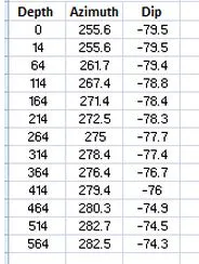
我希望能够使用方向和距离绘制两条线。这是钻孔追踪数据，目前我的数据格式如下：

深度实际上是井孔的距离，而不是垂直深度。方位角是相对于磁北方向的。倾角基于0为水平。我想从同一点（0,0,0可以）绘制两条线，并根据这种信息查看它们的差异。

我没有使用Matplotlib的经验，但熟悉Python，并希望了解这个绘图工具。我找到了这个页面，它帮助我理解了框架，但我仍然无法弄清如何绘制带有3D向量的线条。有人能给我一些关于如何做这个或者在哪里找到我需要的指导吗？谢谢。

- cndnflyr

---

第一步，也可能是最大的挑战，是找到一种将这些数据转换为笛卡尔坐标的方法。然后，您只需要绘制它们。 - loopbackbee

我希望这是一个相当常见的任务，并且在matplotlib中有一个可用的模块。我已经在2D中使用shapely完成了这个任务，我会看看是否有人制作了一个3D的等效模块。 - cndnflyr

matplotlib支持极坐标，但如果我正确理解您的解释，您需要为每个点移动“中心”，并根据您想要的最终结果的方向对角度进行修正。 - loopbackbee

没错。从0,0,0开始。找到下一个坐标，它在水平面上是255.6°，在水平面下方79.5°，距离0,0,0有14米。然后从找到的那个坐标开始，再找下一个，以此类推... - cndnflyr

看看这篇关于球坐标和转换为笛卡尔坐标的沃尔夫勒姆文章，可能会有用... - MattDMo

Answer 1

一个脚本将您的坐标转换为笛卡尔坐标，并使用matplotlib进行绘图，包括注释：

import numpy as np
import matplotlib.pyplot as plt
# import for 3d plot
from mpl_toolkits.mplot3d import Axes3D
# initializing 3d plot
fig = plt.figure()
ax = fig.add_subplot(111, projection = '3d')
# several data points 
r = np.array([0, 14, 64, 114])
# get lengths of the separate segments 
r[1:] = r[1:] - r[:-1]
phi = np.array([255.6, 255.6, 261.7, 267.4])
theta = np.array([-79.5, -79.5, -79.4, -78.8])
# convert to radians
phi = phi * 2 * np.pi / 360.
# in spherical coordinates theta is measured from zenith down; you are measuring it from horizontal plane up 
theta = (90. - theta) * 2 * np.pi / 360.
# get x, y, z from known formulae
x = r*np.cos(phi)*np.sin(theta)
y = r*np.sin(phi)*np.sin(theta)
z = r*np.cos(theta)
# np.cumsum is employed to gradually sum resultant vectors 
ax.plot(np.cumsum(x),np.cumsum(y),np.cumsum(z))

- Andrey Sobolev

---

那太棒了！谢谢你。里面有很多内容。这样做所有点的转换然后将它们相加以得到每个坐标是非常聪明的。我仍在思考极坐标系中的phi和theta转换。不过，我不明白r[1:] = r[1:] - r[:-1]是如何工作的。你能详细说明一下吗？ - cndnflyr

@cndnflyr r[1:] = r[1:] - r[:-1]的意思是说[r[n+1] - r[n] for n in range(1,len(r))]，如果这样说更容易理解。简单来说：从r的第二个元素开始，将每个后续元素重新定义为它与原始前一个元素之间的差异。 - Paul H

@Paul 谢谢，这很有帮助。它使用了从原始列表中取出的两个列表，并使用以r[0]开头的列表从以r[1]开头的列表中减去。因为它们的长度相同，所以这样做是可行的。太好了。 - cndnflyr

作为一个奇怪的副作用，r[1:] - r[:-1] 比 np.diff(r) 更快。 - tacaswell

@tcaswell：这可能是由于函数调用开销 - np.diff 是递归的。 - Andrey Sobolev

Answer 2

针对500米深的钻孔，您可以使用最小曲率法，否则位置误差将非常大。我在地质统计的Python模块（PyGSLIB）中实现了这一点。以下是一个示例，展示了真实钻孔数据库的完整测量过程，包括试金石/岩性间隔的位置：

http://nbviewer.ipython.org/github/opengeostat/pygslib/blob/master/pygslib/Ipython_templates/demo_1.ipynb

这还展示了如何将钻孔以VTK格式导出以便在Paraview中加载。

在Paraview中显示的结果

Cython代码来desurvey一个间隔如下：

cpdef dsmincurb( float len12,
                 float azm1,
                 float dip1,
                 float azm2,
                 float dip2):

    """    
    dsmincurb(len12, azm1, dip1, azm2, dip2)

    Desurvey one interval with minimum curvature 

    Given a line with length ``len12`` and endpoints p1,p2 with 
    direction angles ``azm1, dip1, azm2, dip2``, this function returns 
    the differences in coordinate ``dz,dn,de`` of p2, assuming
    p1 with coordinates (0,0,0)

    Parameters
    ----------
    len12, azm1, dip1, azm2, dip2: float
        len12 is the length between a point 1 and a point 2.
        azm1, dip1, azm2, dip2 are direction angles azimuth, with 0 or 
        360 pointing north and dip angles measured from horizontal 
        surface positive downward. All these angles are in degrees.


    Returns
    -------
    out : tuple of floats, ``(dz,dn,de)``
        Differences in elevation, north coordinate (or y) and 
        east coordinate (or x) in an Euclidean coordinate system. 

    See Also
    --------
    ang2cart, 

    Notes
    -----
    The equations were derived from the paper: 
        http://www.cgg.com/data//1/rec_docs/2269_MinimumCurvatureWellPaths.pdf

    The minimum curvature is a weighted mean based on the
    dog-leg (dl) value and a Ratio Factor (rf = 2*tan(dl/2)/dl )
    if dl is zero we assign rf = 1, which is equivalent to  balanced 
    tangential desurvey method. The dog-leg is zero if the direction 
    angles at the endpoints of the desurvey intervals are equal.  

    Example
    --------

    >>> dsmincurb(len12=10, azm1=45, dip1=75, azm2=90, dip2=20)
    (7.207193374633789, 1.0084573030471802, 6.186459064483643)

    """

    # output
    cdef:
        float dz
        float dn
        float de 


    # internal 
    cdef:
        float i1
        float a1
        float i2
        float a2
        float DEG2RAD
        float rf
        float dl

    DEG2RAD=3.141592654/180.0

    i1 = (90 - dip1) * DEG2RAD
    a1 = azm1 * DEG2RAD

    i2 = (90 - dip2) * DEG2RAD
    a2 = azm2 * DEG2RAD

    # calculate the dog-leg (dl) and the Ratio Factor (rf)
    dl = acos(cos(i2-i1)-sin(i1)*sin(i2)*(1-cos(a2-a1))) 

    if dl!=0.: 
        rf = 2*tan(dl/2)/dl  # minimum curvature
    else:
        rf=1                 # balanced tangential



    dz = 0.5*len12*(cos(i1)+cos(i2))*rf
    dn = 0.5*len12*(sin(i1)*cos(a1)+sin(i2)*cos(a2))*rf
    de = 0.5*len12*(sin(i1)*sin(a1)+sin(i2)*sin(a2))*rf

    return dz,dn,de

- Adrian Martínez Vargas

---

整个Python模块可以通过conda进行安装，只需一行代码conda install -c https://conda.binstar.org/opengeostat pygslib。它使用GPL/MIT许可证，并由Opengeostat Consulting开发。 - Adrian Martínez Vargas

这很有趣。你能否将ipynb重新托管到其他地方？ - elmato

当然，IPython和测试数据在这里：https://opengeostat.github.io/pygslib/Tutorial.html。如果您使用pygslib的开发版本运行此代码，则可能需要进行一些更新。 - Adrian Martínez Vargas