如何在Python中绘制ROC曲线

Question

我正在尝试使用逻辑回归软件包在Python中开发的预测模型来绘制ROC曲线以评估模型的准确性。我已经计算出真正例率和假正例率，但是我无法弄清如何使用matplotlib正确绘制这些并计算AUC值。我该怎么做？

- user3847447

Answer 1

以下是两种尝试的方法，假设您的model是一个sklearn预测器：

import sklearn.metrics as metrics
# calculate the fpr and tpr for all thresholds of the classification
probs = model.predict_proba(X_test)
preds = probs[:,1]
fpr, tpr, threshold = metrics.roc_curve(y_test, preds)
roc_auc = metrics.auc(fpr, tpr)

# method I: plt
import matplotlib.pyplot as plt
plt.title('Receiver Operating Characteristic')
plt.plot(fpr, tpr, 'b', label = 'AUC = %0.2f' % roc_auc)
plt.legend(loc = 'lower right')
plt.plot([0, 1], [0, 1],'r--')
plt.xlim([0, 1])
plt.ylim([0, 1])
plt.ylabel('True Positive Rate')
plt.xlabel('False Positive Rate')
plt.show()

# method II: ggplot
from ggplot import *
df = pd.DataFrame(dict(fpr = fpr, tpr = tpr))
ggplot(df, aes(x = 'fpr', y = 'tpr')) + geom_line() + geom_abline(linetype = 'dashed')

或者尝试一下

ggplot(df, aes(x = 'fpr', ymin = 0, ymax = 'tpr')) + geom_line(aes(y = 'tpr')) + geom_area(alpha = 0.2) + ggtitle("ROC Curve w/ AUC = %s" % str(roc_auc)) 

- uniquegino

---

那么，“preds”基本上是您的“predict_proba”分数，“model”是您的分类器？ - Chris Nielsen

@ChrisNielsen preds是y hat；是的，model是经过训练的分类器。 - uniquegino

all thresholds是什么，它们是如何计算的？ - mrgloom

@mrgloom 它们是由sklearn.metrics.roc_curve自动选择的。 - erobertc

Answer 2

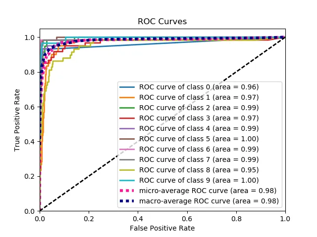
这是绘制ROC曲线的最简单方法，只需要提供一组真实标签和预测概率即可。最棒的是，它可以为所有类别绘制ROC曲线，因此您可以得到多个漂亮的曲线。

import scikitplot as skplt
import matplotlib.pyplot as plt

y_true = # ground truth labels
y_probas = # predicted probabilities generated by sklearn classifier
skplt.metrics.plot_roc_curve(y_true, y_probas)
plt.show()

这是由plot_roc_curve生成的样本曲线。我使用了scikit-learn中的样本数字数据集，因此有10个类别。请注意，为每个类别绘制一个ROC曲线。

免责声明：请注意，此处使用了我开发的scikit-plot库。

- Reii Nakano

---

如何计算 y_true 和 y_probas？ - Md. Rezwanul Haque

Reii Nakano - 你是一个伪装成天使的天才。你让我的一天变得美好。这个程序包非常简单，但效果却非常显著。我完全尊重你。只是关于你上面的代码片段最后一行之前的那行，它不应该是：skplt.metrics.plot_roc_curve(y_true, y_probas)吗？非常感谢你。 - salvu

这应该被选为正确答案！非常有用的包。 - Srivathsa

我使用该软件包时遇到了问题。每次尝试绘制ROC曲线时，它都会报告我有“太多的索引”。我将y_test和pred作为输入提供。我能够得到预测结果，但由于这个错误，无法绘制图形。这是由于我使用的Python版本问题吗？ - Herc01

我必须调整我的 y_pred 数据的大小，使其变为 N×1 的形状，而不仅仅是一个列表：y_pred.reshape(len(y_pred),1)。现在我收到了错误信息“IndexError: index 1 is out of bounds for axis 1 with size 1”，但是画出了一张图，我猜这是因为代码期望二元分类器提供一个 Nx2 的向量，每个类别都有一个概率。 - Vidar

Answer 3

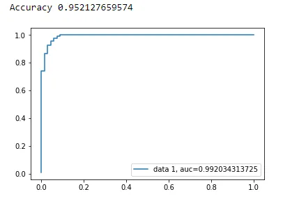
使用matplotlib绘制二元分类的AUC曲线

from sklearn import svm, datasets
from sklearn import metrics
from sklearn.linear_model import LogisticRegression
from sklearn.model_selection import train_test_split
from sklearn.datasets import load_breast_cancer
import matplotlib.pyplot as plt

加载乳腺癌数据集

breast_cancer = load_breast_cancer()

X = breast_cancer.data
y = breast_cancer.target

拆分数据集

X_train, X_test, y_train, y_test = train_test_split(X,y,test_size=0.33, random_state=44)

模型

clf = LogisticRegression(penalty='l2', C=0.1)
clf.fit(X_train, y_train)
y_pred = clf.predict(X_test)

准确性

print("Accuracy", metrics.accuracy_score(y_test, y_pred))

AUC曲线

y_pred_proba = clf.predict_proba(X_test)[::,1]
fpr, tpr, _ = metrics.roc_curve(y_test,  y_pred_proba)
auc = metrics.roc_auc_score(y_test, y_pred_proba)
plt.plot(fpr,tpr,label="data 1, auc="+str(auc))
plt.legend(loc=4)
plt.show()

- ajayramesh

Answer 4

目前还不清楚这里的问题所在，但如果你有一个数组true_positive_rate和一个数组false_positive_rate，那么绘制ROC曲线并获取AUC就像这样简单：

import matplotlib.pyplot as plt
import numpy as np

x = # false_positive_rate
y = # true_positive_rate 

# This is the ROC curve
plt.plot(x,y)
plt.show() 

# This is the AUC
auc = np.trapz(y,x)

- ebarr

---

如果代码中有FPR、TPR的一行简述，那么这个答案会更好。 - aerin

fpr，tpr，threshold = metrics.roc_curve(y_test，preds)意思是计算二分类问题中的ROC曲线和AUC面积。其中，fpr表示假正率（false positive rate），tpr表示真正率（true positive rate），threshold表示分类器阈值的列表。y_test是真实标签，preds是预测的概率分数或决策函数。 - aerin

这里的'metrics'是什么意思？它确切指的是什么？ - dekio

@dekio 这里的'metrics'来自于sklearn：from sklearn import metrics - Baptiste Pouthier

fpr[i]和tpr[i]应该是基于阈值i的假阳性率和真阳性率。fpr是在所有负样本中超过阈值的负样本数量除以所有负样本的数量，而tpr是在所有正样本中超过阈值的正样本数量除以所有正样本的数量。 - undefined

Answer 5

以下是计算ROC曲线（散点图）的Python代码：

import matplotlib.pyplot as plt
import numpy as np

score = np.array([0.9, 0.8, 0.7, 0.6, 0.55, 0.54, 0.53, 0.52, 0.51, 0.505, 0.4, 0.39, 0.38, 0.37, 0.36, 0.35, 0.34, 0.33, 0.30, 0.1])
y = np.array([1,1,0, 1, 1, 1, 0, 0, 1, 0, 1,0, 1, 0, 0, 0, 1 , 0, 1, 0])

# false positive rate
fpr = []
# true positive rate
tpr = []
# Iterate thresholds from 0.0, 0.01, ... 1.0
thresholds = np.arange(0.0, 1.01, .01)

# get number of positive and negative examples in the dataset
P = sum(y)
N = len(y) - P

# iterate through all thresholds and determine fraction of true positives
# and false positives found at this threshold
for thresh in thresholds:
    FP=0
    TP=0
    for i in range(len(score)):
        if (score[i] > thresh):
            if y[i] == 1:
                TP = TP + 1
            if y[i] == 0:
                FP = FP + 1
    fpr.append(FP/float(N))
    tpr.append(TP/float(P))

plt.scatter(fpr, tpr)
plt.show()

- Mona

---

你在内部循环中也使用了相同的“i”外部循环索引。 - Ali Yeşilkanat

参考文献不存在。 - luckydonald

Answer 6

from sklearn import metrics
import numpy as np
import matplotlib.pyplot as plt

y_true = # true labels
y_probas = # predicted results
fpr, tpr, thresholds = metrics.roc_curve(y_true, y_probas, pos_label=0)

# Print ROC curve
plt.plot(fpr,tpr)
plt.show() 

# Print AUC
auc = np.trapz(tpr,fpr)
print('AUC:', auc)

- Cherry Wu

---

如何计算 y_true = #真实标签, y_probas = #预测结果? - Md. Rezwanul Haque

如果您有真实数据，y_true就是您的真实数据（标签），y_probas是您的模型预测的结果。 - Cherry Wu

Answer 7

根据stackoverflow、scikit-learn文档和其他来源的多个评论，我制作了一个Python包，可以以非常简单的方式绘制ROC曲线（和其他指标）。

安装包：pip install plot-metric（更多信息请见本文末尾）

绘制ROC曲线（下面的示例来自文档）：

二分类

我们加载一个简单的数据集并创建训练集和测试集：

from sklearn.datasets import make_classification
from sklearn.model_selection import train_test_split
X, y = make_classification(n_samples=1000, n_classes=2, weights=[1,1], random_state=1)
X_train, X_test, y_train, y_test = train_test_split(X, y, test_size=0.5, random_state=2)

训练分类器并对测试集进行预测：

from sklearn.ensemble import RandomForestClassifier
clf = RandomForestClassifier(n_estimators=50, random_state=23)
model = clf.fit(X_train, y_train)

# Use predict_proba to predict probability of the class
y_pred = clf.predict_proba(X_test)[:,1]

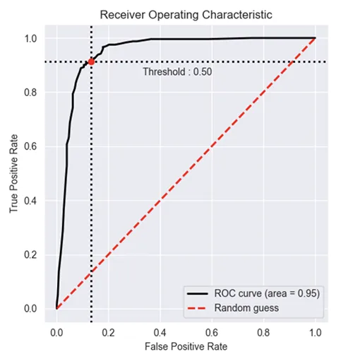
您现在可以使用plot_metric来绘制ROC曲线：

from plot_metric.functions import BinaryClassification
# Visualisation with plot_metric
bc = BinaryClassification(y_test, y_pred, labels=["Class 1", "Class 2"])

# Figures
plt.figure(figsize=(5,5))
bc.plot_roc_curve()
plt.show()

结果 :

您可以在该软件包的Github和文档中找到更多示例：

• Github：https://github.com/yohann84L/plot_metric
• 文档：https://plot-metric.readthedocs.io/en/latest/

- Yohann L.

---

我已经尝试过这个方法，感觉还不错，但似乎只有当分类标签为0或1时才有效，如果我的标签是1和2，它就无法正常工作。你知道如何解决吗？此外，似乎无法编辑图表（如图例）。 - Reut

二元分类需要您手动指定阈值，默认为0.5。如何计算一个不同的、最佳的阈值呢？ - skan

Answer 8

有一个叫做metriculous的库可以为您完成这个任务:

$ pip install metriculous

首先让我们模拟一些数据，通常这些数据来自测试数据集和模型：

import numpy as np

def normalize(array2d: np.ndarray) -> np.ndarray:
    return array2d / array2d.sum(axis=1, keepdims=True)

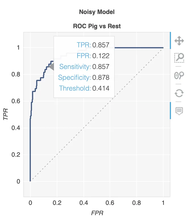
class_names = ["Cat", "Dog", "Pig"]
num_classes = len(class_names)
num_samples = 500

# Mock ground truth
ground_truth = np.random.choice(range(num_classes), size=num_samples, p=[0.5, 0.4, 0.1])

# Mock model predictions
perfect_model = np.eye(num_classes)[ground_truth]
noisy_model = normalize(
    perfect_model + 2 * np.random.random((num_samples, num_classes))
)
random_model = normalize(np.random.random((num_samples, num_classes)))

现在，我们可以使用metriculous生成包含各种指标和图表的表格，包括ROC曲线。

import metriculous

metriculous.compare_classifiers(
    ground_truth=ground_truth,
    model_predictions=[perfect_model, noisy_model, random_model],
    model_names=["Perfect Model", "Noisy Model", "Random Model"],
    class_names=class_names,
    one_vs_all_figures=True, # This line is important to include ROC curves in the output
).save_html("model_comparison.html").display()

输出的ROC曲线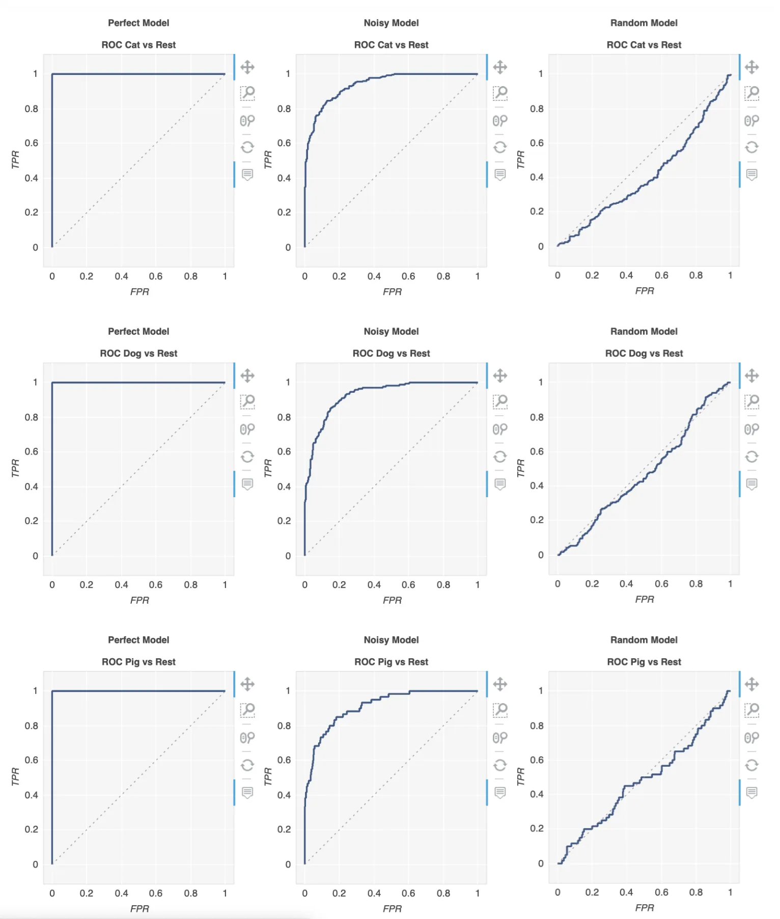： 图表可缩放和拖动，当鼠标悬停在图表上时，您会获得更多细节：

- egdvnyjklu

Answer 9

前面的回答假设您确实自己计算了TP / Sens。手动计算是不好的，容易在计算中出错，最好使用库函数来完成所有这些。

scikit_lean中的plot_roc函数正是您所需要的： http://scikit-learn.org/stable/auto_examples/model_selection/plot_roc.html 代码的关键部分如下：

  for i in range(n_classes):
      fpr[i], tpr[i], _ = roc_curve(y_test[:, i], y_score[:, i])
      roc_auc[i] = auc(fpr[i], tpr[i])

- Max

---

如何计算y_score？ - Saeed

Answer 10

你也可以跟随scikit的官方文档：
https://scikit-learn.org/stable/auto_examples/model_selection/plot_roc.html#sphx-glr-auto-examples-model-selection-plot-roc-py

- PV8