球面上密度最高的位置

Question

球面上密度最高的位置

algorithmmathgeometrycomputational-geometry

5

我有很多点分布在球体表面上。如何计算具有最大点密度的球体区域/点的面积？我需要快速完成这项工作。例如，如果这是一个正方形，我想我可以创建一个网格，然后让点投票哪个部分是最好的。我尝试过将点转换为球坐标，然后做一个网格，但由于极点周围的点在球体上很接近，但在变换后距离较远，所以这并不有效。谢谢。

- Johan

尝试根据纬度为点分配权重。 - n. m.

1

@Johan：线性时间。将您的点投影到xy平面、xz平面和yz平面上，并将其捕捉到网格上。对于每个平面中的每个网格单元格，制作一个三角形列表，当投影时击中该网格单元格。如果您的网格粗糙度与三角形大小大致相同，则最小的三个单元格将包含恒定数量的三角形；使用它。 - tmyklebu

Tmyklebu的建议，就像Darren Engwirda的答案一样，引入了一个需要纠正的偏差。这个修正涉及计算一些小球三角形的面积，可以使用高斯-波涅特公式和一些三角学来完成，或者通过计算投影映射的Jacobian来近似计算。我建议使用一种避免引入这种偏差的方法。 - Douglas Zare

你在几个地方又错了。偏差不小。球面三角形的面积和空间中的面积之间的差异可能相当大。如果你谷歌球面三角形的面积，第一个搜索结果是沃尔夫勒姆数学世界的页面，给出了我所说的角度缺陷、高斯-波内特公式的面积。这需要你计算一些球面角度，它们与3D角度不同，我敢打赌大多数人会在相当复杂的计算中犯错。所以，如果你真的想实现这个功能，我建议避免导致这种偏差的方法。 - Douglas Zare

如果计算球面面积很容易，那么检查一下你关于偏差很小的说法是错误的。使用更大的相对误差的二十面体细分可以使面积扭曲1.584倍。我不知道你从哪里得出了epsilon+O(epsilon^2)，但是从球面三角形的面积到空间三角形的面积没有这样的界限。空间中的三角形可以具有面积为1，而球面三角形的面积可以任意接近0。sds和george等人的方法比尝试进行球面三角测量更简单、更少出错。 - Douglas Zare

显示剩余8条评论

10个回答

4

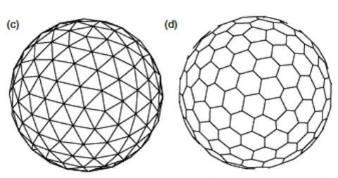
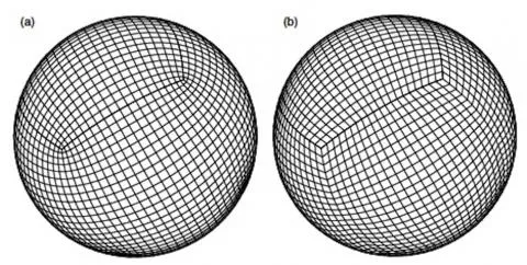
要添加其他替代方案：可以通过细化内切多面体在球状几何上定义许多（几乎）正则网格。第一个选项称为二十面体网格，它是球面表面的三角剖分。通过连接每个顶点周围的三角形的中心，还可以创建基于底层三角剖分的双重六边形网格。

icosahedral grid

如果你不喜欢三角形（和/或六边形），另一种选择是立方体球面网格，它由划分内接立方体的各个面并将结果投影到球面上形成：

enter image description here

无论哪种情况，重要的是所得到的网格几乎是规则的——因此，为了评估球体上密度最高的区域，您可以简单地执行直方图样式的分析，计算每个网格单元格中的样本数量。

正如一些评论者指出的那样，为了考虑网格中轻微的不规则性，可以通过将每个网格单元格的面积除以其面积来归一化直方图计数。然后，得到的密度被给定为“每单位面积”的度量。要计算每个网格单元格的面积，有两个选择：（i）可以通过假设边缘是直线来计算每个单元格的“平坦”面积——当网格足够密集时，这种近似可能相当好，或者（ii）可以通过评估必要的曲面积分来计算“真实”的表面积。

如果您有兴趣有效地执行必要的“点-在-单元格”查询，一种方法是将网格构造为quadtree——从粗略内接多面体开始，将其面细化为子面的树。要查找包含单元格，只需从根遍历树即可，这通常是一个O(log(n))操作。

你可以在这里获取一些有关这些网格类型的附加信息here。

- Darren Engwirda

2

“立方体”选项似乎不能保留区域，因此会引入需要纠正的偏差。 - user1196549

这些图片很漂亮，但是公式却缺失了。你如何确定一个特定的向量属于特定的域？ - sds

@sds：在立方体投影的情况下，您将点投影到立方体上。在测地线镶嵌的情况下，您仍然可以将点投影到立方体上，然后像我在评论中提到的那样进行O（1）点三角形测试。唯一真正缺少的是Yves Daoust指出的归一化问题。 - tmyklebu

2

把球面上的点视为3D点可能并不糟糕。

尝试以下两种方法之一：

1.选择k，在数据或所选兴趣点中进行近似k-NN搜索，然后按它们到查询点的距离加权结果。针对不同近似k-NN算法复杂度可能各不相同。

2.构建空间划分数据结构如k-d树，然后在数据或所选兴趣点周围以球形范围进行近似(或精确)区域计数查询。对于每个近似范围查询及其最先进的算法，复杂度为O(log(n)+epsilon^(-3))或O(epsilon^(-3)*log(n))，其中epsilon是与查询球大小有关的范围误差阈值。对于精确范围查询，每个查询的复杂度为O(n^(2/3))。

- user3784553

2

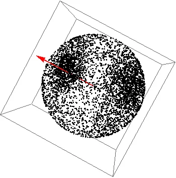
将球面划分为相等面积的区域（由纬线和经线界定），如我在那里的回答中描述，并计算每个区域内的点数。

当N~M时，各区域的长宽比率将不均匀（赤道附近的区域更加“正方形”，而极地附近的区域则更加细长）。这并不是问题，因为随着N和M的增加，各区域的直径趋近于0。这种方法的计算简便性胜过其他优秀答案中具有美丽图片的更好的域均匀性。

一种简单的修改方法是，在链接回答中描述的N*M个区域中添加两个“极点”区域以提高数字稳定性（当点非常接近极点时，其经度不确定）。这样可以限制各区域的长宽比率。

- sds

将区域的直径趋近于零并不是一个足够强的保证；你需要在适度的网格尺寸下将它们限制得足够接近于零，因为过细的网格实际上只会挑选出一些偶然的噪声分布。如果你选择这条路线，分别铺设极地帽子是一个好主意，但在那个阶段，你更接近于达伦·恩格维尔达的第二个答案。 - tmyklebu

1

你可以使用彼得斯投影，这种投影方式可以保留区域信息。

这将使您能够高效地计算网格中的点数，还可以使用积分图像技巧在滑动窗口（盒式帕尔泽窗口）中进行计数。

- user1196549

有趣。在网格上投影的正方形会对应到球体上的什么？它们看起来会相似吗？ - Johan

想象一张由等距子午线和平行线形成的网格，随着接近极地，平行线之间的间距越来越大。 - user1196549

0

如果我理解正确，您正在尝试在球体上找到密集点。

如果某些点更密集

考虑笛卡尔坐标并找到点的平均X、Y、Z
找到距离平均X、Y、Z最近的在球体上的点（您可以考虑使用球面坐标，只需将半径延伸到原始半径）。

约束条件

如果平均X、Y、Z与中心之间的距离小于r/2，则此算法可能无法按预期工作。

- fermat4214

0

我不是数学大师，但也许可以通过分析的方式解决：

1. 缩短坐标

2. R = (Σ（n=0. n=max）（Σ（m=0. M=n）（1/A^diff_in_consecative）*angle）/Σangle

A = 任何常数

- Naresh Teli

0

如果您想要一个最大密度的径向区域，这就是具有 k = 1 和 dist(a, b) = great circle distance (a, b) 的强健磁盘覆盖问题（请参见https://en.wikipedia.org/wiki/Great-circle_distance）。

https://www4.comp.polyu.edu.hk/~csbxiao/paper/2003%20and%20before/PDCS2003.pdf

- DoctorPangloss

0

这实际上只是我之前this答案的倒置

只需将等距球面顶点的方程反转为表面单元格索引。不要尝试将单元格可视化为除圆形外的其他形状，否则你会发疯的。但如果有人真的这样做了，请在此处发布结果（并让我知道）

现在只需创建2D单元格地图，并在O(N)中进行密度计算（类似于直方图），与Darren Engwirda在他的答案中提出的类似。

这是C ++代码的外观

//---------------------------------------------------------------------------
const int na=16;                                // sphere slices
      int nb[na];                           // cells per slice
const int na2=na<<1;
      int map[na][na2];                     // surface cells
const double da=M_PI/double(na-1);          // latitude angle step
      double db[na];                        // longitude angle step per slice
// sherical -> orthonormal
void abr2xyz(double &x,double &y,double &z,double a,double b,double R)
    {
    double r;
    r=R*cos(a);
    z=R*sin(a);

    y=r*sin(b);
    x=r*cos(b);
    }
// sherical -> surface cell
void ab2ij(int &i,int &j,double a,double b)
    {
    i=double(((a+(0.5*M_PI))/da)+0.5);
    if (i>=na) i=na-1;
    if (i<  0) i=0;
    j=double(( b            /db[i])+0.5);
    while (j<     0) j+=nb[i];
    while (j>=nb[i]) j-=nb[i];
    }
// sherical <- surface cell
void ij2ab(double &a,double &b,int i,int j)
    {
    if (i>=na) i=na-1;
    if (i<  0) i=0;
    a=-(0.5*M_PI)+(double(i)*da);
    b=             double(j)*db[i];
    }
// init variables and clear map
void ij_init()
    {
    int i,j;
    double a;
    for (a=-0.5*M_PI,i=0;i<na;i++,a+=da)
        {
        nb[i]=ceil(2.0*M_PI*cos(a)/da);     // compute actual circle cell count
        if (nb[i]<=0) nb[i]=1;
        db[i]=2.0*M_PI/double(nb[i]);       // longitude angle step
        if ((i==0)||(i==na-1)) { nb[i]=1; db[i]=1.0; }
        for (j=0;j<na2;j++) map[i][j]=0;    // clear cell map
        }
    }
//---------------------------------------------------------------------------
// this just draws circle from point x0,y0,z0 with normal nx,ny,nz and radius r
// need some vector stuff of mine so i did not copy the body here (it is not important)
void glCircle3D(double x0,double y0,double z0,double nx,double ny,double nz,double r,bool _fill);
//---------------------------------------------------------------------------
void analyse()
    {
    // n is number of points and r is just visual radius of sphere for rendering
    int i,j,ii,jj,n=1000;
    double x,y,z,a,b,c,cm=1.0/10.0,r=1.0;
    // init
    ij_init();      // init variables and map[][]
    RandSeed=10;    // just to have the same random points generated every frame (do not need to store them)
    // generate draw and process some random surface points
    for (i=0;i<n;i++)
        {
        a=M_PI*(Random()-0.5);
        b=M_PI* Random()*2.0 ;
        ab2ij(ii,jj,a,b);       // cell corrds
        abr2xyz(x,y,z,a,b,r);   // 3D orthonormal coords
        map[ii][jj]++; // update cell density
        // this just draw the point (x,y,z) as line in OpenGL so you can ignore this
        double w=1.1;   // w-1.0 is rendered line size factor
        glBegin(GL_LINES);
        glColor3f(1.0,1.0,1.0); glVertex3d(x,y,z);
        glColor3f(0.0,0.0,0.0); glVertex3d(w*x,w*y,w*z);
        glEnd();
        }

    // draw cell grid (color is function of density)
    for (i=0;i<na;i++)
     for (j=0;j<nb[i];j++)
        {
        ij2ab(a,b,i,j); abr2xyz(x,y,z,a,b,r);
        c=map[i][j]; c=0.1+(c*cm); if (c>1.0) c=1.0;
        glColor3f(0.2,0.2,0.2); glCircle3D(x,y,z,x,y,z,0.45*da,0); // outline
        glColor3f(0.1,0.1,c  ); glCircle3D(x,y,z,x,y,z,0.45*da,1); // filled by bluish color the more dense the cell the more bright it is
        }
    }
//---------------------------------------------------------------------------

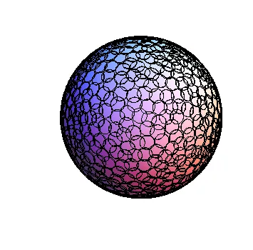
结果看起来像这样：

surface density

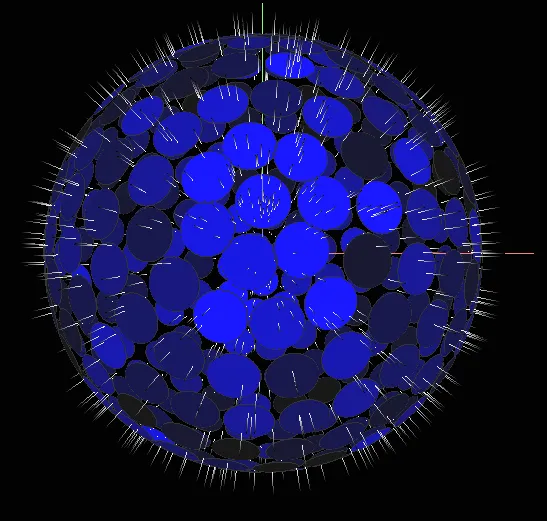
现在只需查看map[][]数组中的内容，您就可以找到密度的全局/局部最小值/最大值或其他任何您需要的值... 只是不要忘记，大小为map[na][nb[i]]，其中i是数组中的第一个索引。网格大小由na常量控制，cm只是密度到颜色比例...

[edit1]得到了四重网格，这是使用映射的远远更准确的表示

surface density

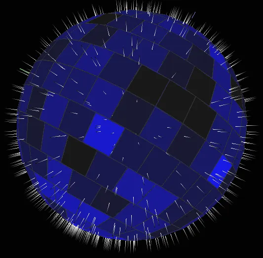
这是关于编程的内容，当na=16时，最严重的舍入误差出现在极点上。如果你想要更精确，可以根据单元格表面积加权密度。对于所有非极点单元格，它都是简单的四边形。对于极点，它是三角扇形（正多边形）。

这是网格绘制代码：

// draw cell quad grid (color is function of density)
int i,j,ii,jj;
double x,y,z,a,b,c,cm=1.0/10.0,mm=0.49,r=1.0;
double dx=mm*da,dy;
for (i=1;i<na-1;i++)    // ignore poles
 for (j=0;j<nb[i];j++)
    {
    dy=mm*db[i];
    ij2ab(a,b,i,j);
    c=map[i][j]; c=0.1+(c*cm); if (c>1.0) c=1.0;
    glColor3f(0.2,0.2,0.2);
    glBegin(GL_LINE_LOOP);
    abr2xyz(x,y,z,a-dx,b-dy,r); glVertex3d(x,y,z);
    abr2xyz(x,y,z,a-dx,b+dy,r); glVertex3d(x,y,z);
    abr2xyz(x,y,z,a+dx,b+dy,r); glVertex3d(x,y,z);
    abr2xyz(x,y,z,a+dx,b-dy,r); glVertex3d(x,y,z);
    glEnd();
    glColor3f(0.1,0.1,c  );
    glBegin(GL_QUADS);
    abr2xyz(x,y,z,a-dx,b-dy,r); glVertex3d(x,y,z);
    abr2xyz(x,y,z,a-dx,b+dy,r); glVertex3d(x,y,z);
    abr2xyz(x,y,z,a+dx,b+dy,r); glVertex3d(x,y,z);
    abr2xyz(x,y,z,a+dx,b-dy,r); glVertex3d(x,y,z);
    glEnd();
    }
i=0; j=0; ii=i+1; dy=mm*db[ii];
ij2ab(a,b,i,j); c=map[i][j]; c=0.1+(c*cm); if (c>1.0) c=1.0;
glColor3f(0.2,0.2,0.2);
glBegin(GL_LINE_LOOP);
for (j=0;j<nb[ii];j++) { ij2ab(a,b,ii,j); abr2xyz(x,y,z,a-dx,b-dy,r); glVertex3d(x,y,z); }
glEnd();
glColor3f(0.1,0.1,c  );
glBegin(GL_TRIANGLE_FAN);                 abr2xyz(x,y,z,a   ,b   ,r); glVertex3d(x,y,z);
for (j=0;j<nb[ii];j++) { ij2ab(a,b,ii,j); abr2xyz(x,y,z,a-dx,b-dy,r); glVertex3d(x,y,z); }
glEnd();
i=na-1; j=0; ii=i-1; dy=mm*db[ii];
ij2ab(a,b,i,j); c=map[i][j]; c=0.1+(c*cm); if (c>1.0) c=1.0;
glColor3f(0.2,0.2,0.2);
glBegin(GL_LINE_LOOP);
for (j=0;j<nb[ii];j++) { ij2ab(a,b,ii,j); abr2xyz(x,y,z,a-dx,b+dy,r); glVertex3d(x,y,z); }
glEnd();
glColor3f(0.1,0.1,c  );
glBegin(GL_TRIANGLE_FAN);                 abr2xyz(x,y,z,a   ,b   ,r); glVertex3d(x,y,z);
for (j=0;j<nb[ii];j++) { ij2ab(a,b,ii,j); abr2xyz(x,y,z,a-dx,b+dy,r); glVertex3d(x,y,z); }
glEnd();

mm 是网格单元大小，mm=0.5 表示完整的单元大小，较小的值会在单元之间创建空间。

- Spektre

-1

考虑使用地理方法来解决这个问题。GIS工具、SQL中的地理数据类型等都可以处理椭球体的曲率。如果您不是在地球上实际建模，可能需要找到一个使用纯球体而不是类似地球的椭球体的坐标系统。

为了提高速度，如果您有大量点并想要它们的最密集位置，栅格热图类型的解决方案可能很有效。您可以创建低分辨率的栅格图像，然后缩放到高密度区域并创建您关心的更高分辨率的单元格。

- user15741

网页内容由stack overflow 提供, 点击上面的

可以查看英文原文，
原文链接

- agentp · Accepted Answer

事实上，将球体分割为规则的非重叠网格没有真正的理由，可以尝试以下方法：

将球体分割为半重叠的圆
参考以下链接生成均匀分布的点（即圆心）：在球面上均匀地分散n个点
通过简单的点积可以非常快速地识别每个圆中的点。如果一些点被重复计算，也并不重要，拥有最多点数的圆仍然代表着最高密度。

enter image description here

Mathematica 实现

对于5000个点，此方法需要12秒进行分析。（编写时间约为10分钟）

 testcircles = { RandomReal[ {0, 1}, {3}] // Normalize};
 Do[While[ (test = RandomReal[ {-1, 1}, {3}] // Normalize ;
     Select[testcircles , #.test > .9 & , 1] ) == {} ];
        AppendTo[testcircles, test];, {2000}];
 vmax = testcircles[[First@
    Ordering[-Table[ 
        Count[ (testcircles[[i]].#) & /@ points   , x_ /; x > .98 ] ,
              {i, Length[testcircles]}], 1]]];

enter image description here