如何在Python中应用分段线性拟合?

86

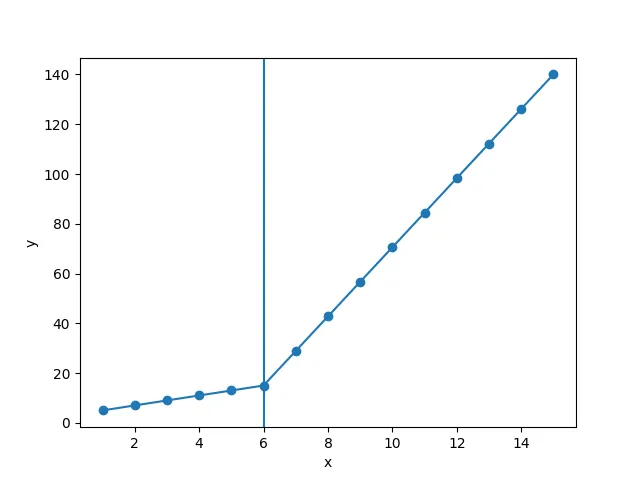
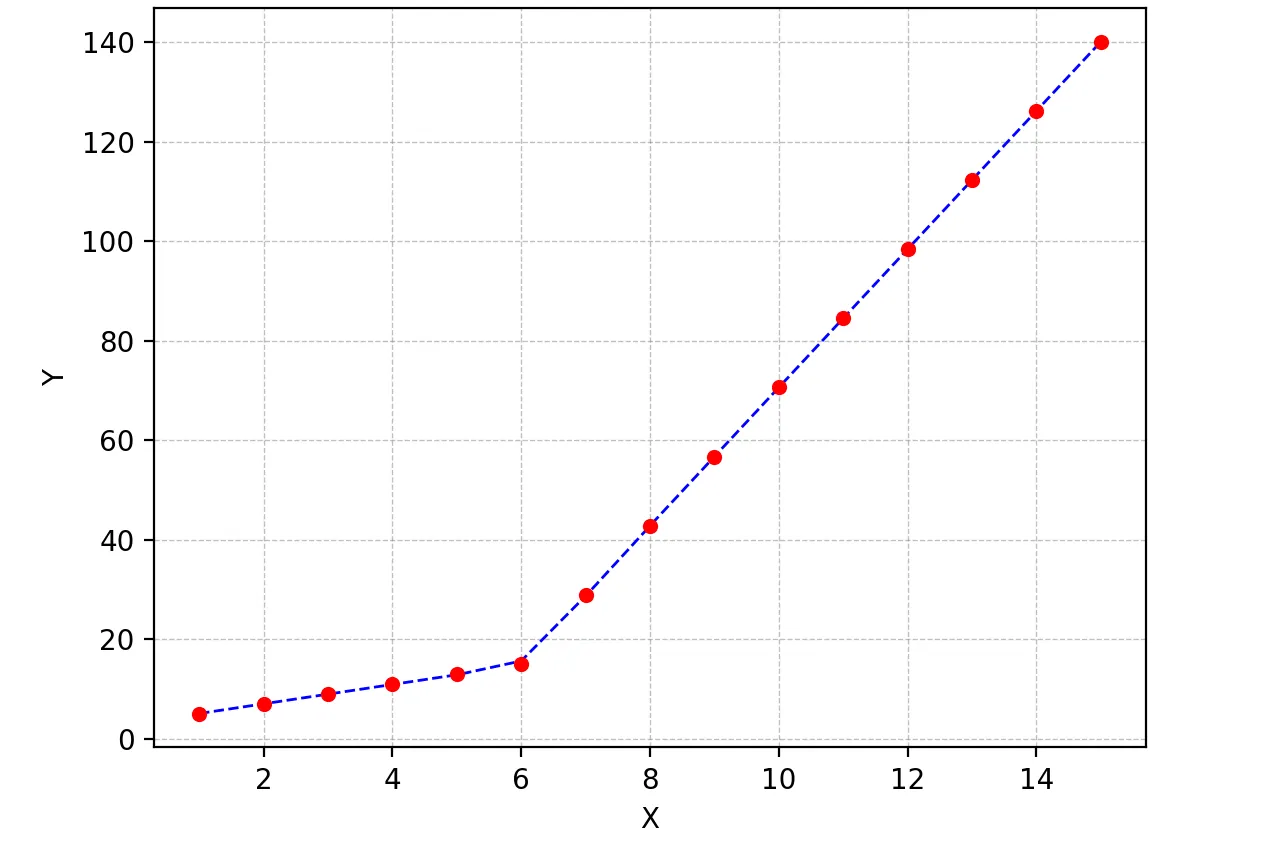
我正在尝试为一个数据集拟合分段线性拟合,如图1所示。

enter image description here

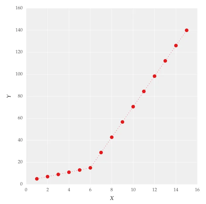
这个图是通过在线上设置得到的。我尝试使用以下代码应用分段线性拟合:

from scipy import optimize
import matplotlib.pyplot as plt
import numpy as np


x = np.array([1, 2, 3, 4, 5, 6, 7, 8, 9, 10 ,11, 12, 13, 14, 15])
y = np.array([5, 7, 9, 11, 13, 15, 28.92, 42.81, 56.7, 70.59, 84.47, 98.36, 112.25, 126.14, 140.03])


def linear_fit(x, a, b):
    return a * x + b
fit_a, fit_b = optimize.curve_fit(linear_fit, x[0:5], y[0:5])[0]
y_fit = fit_a * x[0:7] + fit_b
fit_a, fit_b = optimize.curve_fit(linear_fit, x[6:14], y[6:14])[0]
y_fit = np.append(y_fit, fit_a * x[6:14] + fit_b)


figure = plt.figure(figsize=(5.15, 5.15))
figure.clf()
plot = plt.subplot(111)
ax1 = plt.gca()
plot.plot(x, y, linestyle = '', linewidth = 0.25, markeredgecolor='none', marker = 'o', label = r'\textit{y_a}')
plot.plot(x, y_fit, linestyle = ':', linewidth = 0.25, markeredgecolor='none', marker = '', label = r'\textit{y_b}')
plot.set_ylabel('Y', labelpad = 6)
plot.set_xlabel('X', labelpad = 6)
figure.savefig('test.pdf', box_inches='tight')
plt.close()    

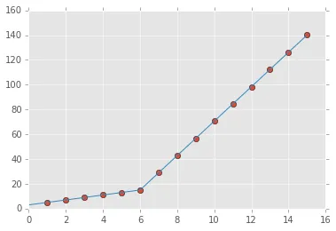
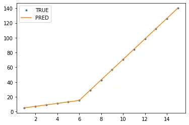
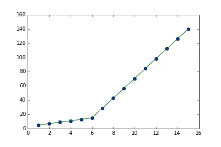
但是这让我得到了图2中的形式拟合,我尝试改变值但是没有任何变化,我无法得到上线的适当匹配。对我来说最重要的要求是如何让Python获取梯度变化点。本质上,我想让Python在适当的范围内识别和拟合两个线性拟合。这在Python中怎么做?
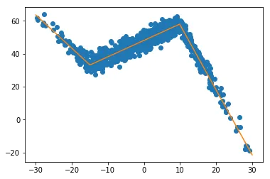
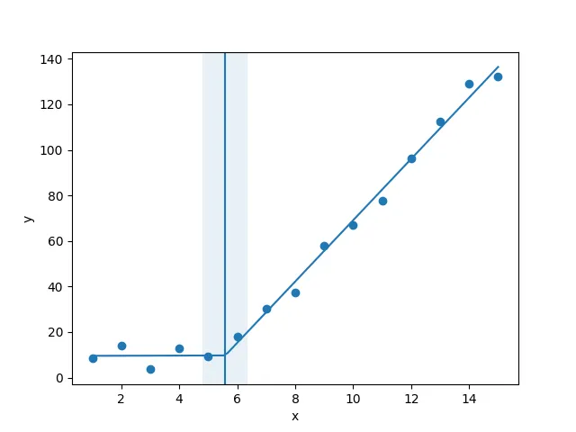
12个回答

83

你可以使用 numpy.piecewise() 创建分段函数,然后使用 curve_fit(),以下是代码

from scipy import optimize
import matplotlib.pyplot as plt
import numpy as np
%matplotlib inline

x = np.array([1, 2, 3, 4, 5, 6, 7, 8, 9, 10 ,11, 12, 13, 14, 15], dtype=float)
y = np.array([5, 7, 9, 11, 13, 15, 28.92, 42.81, 56.7, 70.59, 84.47, 98.36, 112.25, 126.14, 140.03])

def piecewise_linear(x, x0, y0, k1, k2):
    return np.piecewise(x, [x < x0], [lambda x:k1*x + y0-k1*x0, lambda x:k2*x + y0-k2*x0])

p , e = optimize.curve_fit(piecewise_linear, x, y)
xd = np.linspace(0, 15, 100)
plt.plot(x, y, "o")
plt.plot(xd, piecewise_linear(xd, *p))

输出:

在这里输入图片描述

对于 N 零件的配合,请参考 segments_fit.ipynb


33
我该如何将这个扩展成三个部分? - Tom Kurushingal
由于我对错误感兴趣,我使用x = np.random.normal(7,5,15)y= piecewise_linear(x, 5.5,10,0.5,10) +np.random.normal(0,3,x.size)生成了一些带有噪声的点。样本的端点对斜率有很大的影响。 - undefined
由于参数的初始猜测是[1,1,1,1],在其他数据的情况下可能无法收敛到一个良好的拟合结果——它将寻找通过点(1,1)附近的局部最优解。也许考虑选择一个更合理的初始点,如p, e = optimize.curve_fit(piecewise_linear, x, y, p0=[x.mean(), y.mean(),0,0]) - undefined

33
您可以使用pwlf在Python中执行连续分段线性回归。您可以通过使用pip安装此库

在pwlf中,有两种方法可以执行拟合:

  1. 您可以适应指定数量的线段。
  2. 您可以指定应终止连续分段线的x位置。

让我们采用第一种方法,因为它更容易,并且将识别您感兴趣的“梯度变化点”。

当查看数据时,我注意到两个明显的区域。因此,使用两条线段找到最佳可能的连续分段线是有意义的。这是第一种方法。

import numpy as np
import matplotlib.pyplot as plt
import pwlf

x = np.array([1, 2, 3, 4, 5, 6, 7, 8, 9, 10, 11, 12, 13, 14, 15])
y = np.array([5, 7, 9, 11, 13, 15, 28.92, 42.81, 56.7, 70.59,
              84.47, 98.36, 112.25, 126.14, 140.03])

my_pwlf = pwlf.PiecewiseLinFit(x, y)
breaks = my_pwlf.fit(2)
print(breaks)

[1. 5.99819559 15.]

第一条线段的起点为[1., 5.99819559],而第二条线段的起点为[5.99819559, 15.]。因此,您所询问的梯度变化点是5.99819559。

我们可以使用预测函数来绘制这些结果。

x_hat = np.linspace(x.min(), x.max(), 100)
y_hat = my_pwlf.predict(x_hat)

plt.figure()
plt.plot(x, y, 'o')
plt.plot(x_hat, y_hat, '-')
plt.show()

拟合结果图


28

你可以使用样条插值方案来进行分段线性插值,并找到曲线的转折点。二阶导数在转折点处最大(对于单调递增的曲线),可以通过高于2阶的样条插值进行计算。

import numpy as np
import matplotlib.pyplot as plt
from scipy import interpolate

x = np.array([1, 2, 3, 4, 5, 6, 7, 8, 9, 10 ,11, 12, 13, 14, 15])
y = np.array([5, 7, 9, 11, 13, 15, 28.92, 42.81, 56.7, 70.59, 84.47, 98.36, 112.25, 126.14, 140.03])

tck = interpolate.splrep(x, y, k=2, s=0)
xnew = np.linspace(0, 15)

fig, axes = plt.subplots(3)

axes[0].plot(x, y, 'x', label = 'data')
axes[0].plot(xnew, interpolate.splev(xnew, tck, der=0), label = 'Fit')
axes[1].plot(x, interpolate.splev(x, tck, der=1), label = '1st dev')
dev_2 = interpolate.splev(x, tck, der=2)
axes[2].plot(x, dev_2, label = '2st dev')

turning_point_mask = dev_2 == np.amax(dev_2)
axes[2].plot(x[turning_point_mask], dev_2[turning_point_mask],'rx',
             label = 'Turning point')
for ax in axes:
    ax.legend(loc = 'best')

plt.show()

拐点和分段线性插值


13

输入图像描述

此方法使用Scikit-Learn应用分段线性回归。 如果您的点受到噪声影响,可以使用此方法。 它比执行巨大的优化任务(例如来自 scip.optimize 的任何内容,如具有超过3个参数的 curve_fit)更快速,显着更健壮和更通用

import numpy as np
import matplotlib.pylab as plt
from sklearn.tree import DecisionTreeRegressor
from sklearn.linear_model import LinearRegression

# parameters for setup
n_data = 20

# segmented linear regression parameters
n_seg = 3

np.random.seed(0)
fig, (ax0, ax1) = plt.subplots(1, 2)

# example 1
#xs = np.sort(np.random.rand(n_data))
#ys = np.random.rand(n_data) * .3 + np.tanh(5* (xs -.5))

# example 2
xs = np.linspace(-1, 1, 20)
ys = np.random.rand(n_data) * .3 + np.tanh(3*xs)

dys = np.gradient(ys, xs)

rgr = DecisionTreeRegressor(max_leaf_nodes=n_seg)
rgr.fit(xs.reshape(-1, 1), dys.reshape(-1, 1))
dys_dt = rgr.predict(xs.reshape(-1, 1)).flatten()

ys_sl = np.ones(len(xs)) * np.nan
for y in np.unique(dys_dt):
    msk = dys_dt == y
    lin_reg = LinearRegression()
    lin_reg.fit(xs[msk].reshape(-1, 1), ys[msk].reshape(-1, 1))
    ys_sl[msk] = lin_reg.predict(xs[msk].reshape(-1, 1)).flatten()
    ax0.plot([xs[msk][0], xs[msk][-1]],
             [ys_sl[msk][0], ys_sl[msk][-1]],
             color='r', zorder=1)

ax0.set_title('values')
ax0.scatter(xs, ys, label='data')
ax0.scatter(xs, ys_sl, s=3**2, label='seg lin reg', color='g', zorder=5)
ax0.legend()

ax1.set_title('slope')
ax1.scatter(xs, dys, label='data')
ax1.scatter(xs, dys_dt, label='DecisionTree', s=2**2)
ax1.legend()

plt.show()

它是如何工作的

  • 在每个点计算斜率
  • 使用决策树(右图)将相似的斜率分组
  • 对原始数据中的每个组执行线性回归

这是一个非常好的方法。需要进行一些修改才能运行。1:定义n_datan_seg(并使用n_data来生成xs)。2:最好指定导入。 - zgana
有没有一种自动化 n_seg 的方法,使其将数据分成最优分段的数量? - Dante van der Heijden
有没有办法使其适应分段连续线性模型? - undefined

7
一个有两个变化点的示例。如果需要,可以基于此示例测试更多的变化点。
np.random.seed(9999)
x = np.random.normal(0, 1, 1000) * 10
y = np.where(x < -15, -2 * x + 3 , np.where(x < 10, x + 48, -4 * x + 98)) + np.random.normal(0, 3, 1000)
plt.scatter(x, y, s = 5, color = u'b', marker = '.', label = 'scatter plt')

def piecewise_linear(x, x0, x1, b, k1, k2, k3):
    condlist = [x < x0, (x >= x0) & (x < x1), x >= x1]
    funclist = [lambda x: k1*x + b, lambda x: k1*x + b + k2*(x-x0), lambda x: k1*x + b + k2*(x-x0) + k3*(x - x1)]
    return np.piecewise(x, condlist, funclist)

p , e = optimize.curve_fit(piecewise_linear, x, y)
xd = np.linspace(-30, 30, 1000)
plt.plot(x, y, "o")
plt.plot(xd, piecewise_linear(xd, *p))

enter image description here


7
你正在寻找线性树。它们是一种应用分段线性拟合的最佳方法,可以在广义和自动化的方式下进行(也适用于多元和分类环境)。 线性树不同于决策树,因为它们计算线性逼近(而不是常数逼近),并在叶子节点中拟合简单的线性模型。
对于我的一个项目,我开发了linear-tree一个构建带有线性模型的模型树的Python库。

enter image description here

linear-tree被开发成能够完全集成到scikit-learn中。
from sklearn.linear_model import *
from lineartree import LinearTreeRegressor, LinearTreeClassifier

# REGRESSION
regr = LinearTreeRegressor(base_estimator=LinearRegression())
regr.fit(X, y)

# CLASSIFICATION
clf = LinearTreeClassifier(base_estimator=RidgeClassifier())
clf.fit(X, y)

LinearTreeRegressorLinearTreeClassifier作为scikit-learn的BaseEstimator提供。它们是包装器,通过在数据上拟合来自sklearn.linear_model的线性估计器构建决策树。所有在sklearn.linear_model中可用的模型都可以用作线性估计器。

将决策树与线性树进行比较:

enter image description here

enter image description here

考虑到您的数据,概括非常简单明了:

from sklearn.linear_model import LinearRegression
from lineartree import LinearTreeRegressor
import numpy as np
import matplotlib.pyplot as plt

X = np.array(
    [1, 2, 3, 4, 5, 6, 7, 8, 9, 10 ,11, 12, 13, 14, 15]
    ).reshape(-1,1)
y = np.array(
    [5, 7, 9, 11, 13, 15, 28.92, 42.81, 56.7, 70.59, 84.47, 98.36, 112.25, 126.14, 140.03]
    )

model = LinearTreeRegressor(base_estimator=LinearRegression())
model.fit(X, y)

plt.plot(X, y, ".", label='TRUE')
plt.plot(X, model.predict(X), label='PRED')
plt.legend()

enter image description here


4
这句话的意思是:“piecewise-regression python package 正好处理这个问题。”
import numpy as np
import matplotlib.pyplot as plt
import piecewise_regression

x = np.array([1, 2, 3, 4, 5, 6, 7, 8, 9, 10 ,11, 12, 13, 14, 15])
y = np.array([5, 7, 9, 11, 13, 15, 28.92, 42.81, 56.7, 70.59, 84.47, 98.36, 112.25, 126.14, 140.03])

pw_fit = piecewise_regression.Fit(x, y, n_breakpoints=1)
pw_fit.plot()
plt.xlabel("x")
plt.ylabel("y")
plt.show()

piecewise-regression fit

它还提供了拟合结果的信息:
pw_fit.summary()

Statistical summary of the fit

它通过实现Muggeo的迭代算法工作。这里有更多的代码示例 带噪声的例子。为了一个更有趣的例子,我们可以给y数据添加一些噪声并再次进行拟合:
y += np.random.normal(size=len(y)) * 5

pw_fit = piecewise_regression.Fit(x, y, n_breakpoints=1)
pw_fit.plot()

enter image description here


1
https://github.com/chasmani/piecewise-regression 很棒。看到数据+噪声示例的摘要会很有趣。 - undefined

3
使用 numpy.interp 函数,它能够返回给定数据点的函数的一维分段线性插值。

6
这个回答没有解决本质问题:“我希望Python能够在适当的范围内识别和拟合两个线性拟合。这该如何在Python中实现?”numpy.interp只是连接点,但它不会应用拟合。对于所提供的示例,结果恰好相同,但一般情况下并非如此。 - kadee

2

我认为来自scipy.interpolateUnivariateSpline将提供最简单且很可能是最快的分段拟合方式。为了加入一些背景信息,样条是由多项式分段定义的函数。在您的情况下,您正在寻找一个线性样条,其由UnivariateSpline中的k = 1定义。此外,s = 0.5是一个平滑因子,它表示拟合的好坏程度(请查看文档以获取更多信息)。

import numpy as np
import matplotlib.pyplot as plt
from scipy.interpolate import UnivariateSpline

x = np.array([1, 2, 3, 4, 5, 6, 7, 8, 9, 10, 11, 12, 13, 14, 15])
y = np.array([5, 7, 9, 11, 13, 15, 28.92, 42.81, 56.7, 70.59, 84.47, 98.36, 112.25, 126.14, 140.03])


# Solution
spl = UnivariateSpline(x, y, k=1, s=0.5)
xs = np.linspace(x.min(), x.max(), 1000)


fig, ax = plt.subplots()
ax.scatter(x, y, color="red", s=20, zorder=20)
ax.plot(xs, spl(xs), linestyle="--", linewidth=1, color="blue", zorder=10)
ax.grid(color="grey", linestyle="--", linewidth=.5, alpha=.5)
ax.set_ylabel("Y")
ax.set_xlabel("X")
plt.show()

Fitting UnivariateSpline


1

扩展@binoy-pilakkat的答案。

您应该使用numpy.interp

import numpy as np
import matplotlib.pyplot as plt

x = np.array(range(1,16), dtype=float)
y = np.array([5, 7, 9, 11, 13, 15, 28.92,
          42.81, 56.7, 70.59, 84.47,
          98.36, 112.25, 126.14, 140.03], dtype=float)

yinterp = np.interp(x, x, y) # simple as that

plt.plot(x, y, 'bo')
plt.plot(x, yinterp, 'g-')
plt.show()

enter image description here


10
这个回答没有回应核心问题:“我希望Python能够识别和适配两个线性拟合到适当的范围内。在Python中如何实现?” numpy.interp只是连接数据点,但它不会进行拟合。对于提供的示例,结果恰好相同,但一般情况下并非如此。 - kadee

网页内容由stack overflow 提供, 点击上面的
可以查看英文原文,
原文链接