使用SciPy将2D样本集成到矩形网格中

Question

SciPy有三种方法可以对样本进行1D积分（trapz，simps和romb），还有一种方法可以对函数进行2D积分（dblquad），但似乎没有方法可以对样本进行2D积分，即使是在矩形网格上。

我能找到的最接近的方法是scipy.interpolate.RectBivariateSpline.integral - 您可以从矩形网格上的数据创建一个RectBivariateSpline，然后对其进行积分。但是，这并不特别快。

我想要比矩形法更精确的东西（即仅将所有内容相加）。例如，我可以通过创建带有正确权重的数组，将其乘以要积分的数组，然后总结结果来使用2D Simpson's 规则。

但是，如果已经有更好的东西存在，我就不想重新发明轮子。有吗？

- lnmaurer

Answer 1

使用一维规则两次。

>>> from scipy.integrate import simps
>>> import numpy as np
>>> x = np.linspace(0, 1, 20)
>>> y = np.linspace(0, 1, 30)
>>> z = np.cos(x[:,None])**4 + np.sin(y)**2
>>> simps(simps(z, y), x)
0.85134099743259539
>>> import sympy
>>> xx, yy = sympy.symbols('x y')
>>> sympy.integrate(sympy.cos(xx)**4 + sympy.sin(yy)**2, (xx, 0, 1), (yy, 0, 1)).evalf()
0.851349922021627

- pv.

---

好的，对于我的问题，我一直在同一维度的数组上进行积分，因此对我来说更快的方法是为辛普森规则创建一个权重数组（称为simp），然后执行sum（simp * z）--因为我只需要定义simp一次。不过，双重辛普森法也是值得了解的。 - lnmaurer

有没有一种方法可以在三维中实现它？ - chemeng

这是正确的，因为要积分的函数实际上是f（x，y）= g（x）+ h（y），而结果是正确的，因为积分区间为[0,1] x [0,1]。 - David GG

Answer 2

如果您需要处理一个真正的二维矩形积分，那么您会得到类似于这样的东西。

>>> import numpy as np
>>> from scipy.integrate import simps
>>> x_min,x_max,n_points_x = (0,1,50)
>>> y_min,y_max,n_points_y = (0,5,50)
>>> x = np.linspace(x_min,x_max,n_points_x)
>>> y = np.linspace(y_min,y_max,n_points_y)
>>> def F(x,y):
>>>     return x**4 * y
# We reshape to use broadcasting
>>> zz = F(x.reshape(-1,1),y.reshape(1,-1))
>>> zz.shape 
(50,50)
# We first integrate over x and then over y
>>> simps([simps(zz_x,x) for zz_x in zz],y) 
2.50005233

您可以与真实结果进行比较，它是：

- David GG

Answer 3

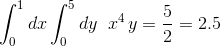
可以通过以下方式在2D中完成。简要绘制一个点阵网格，

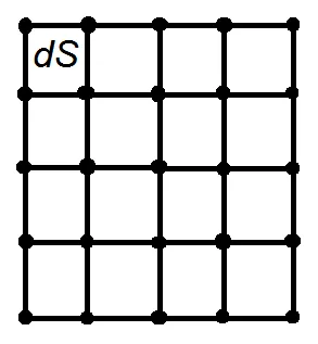
整个网格的积分等于小区域dS的积分之和。梯形法则将小矩形dS上的积分近似为dS的面积乘以dS角落处函数值的平均值，这些角落是网格点：

∫ f(x,y) dS = (f1 + f2 + f3 + f4)/4

其中f1、f2、f3、f4是矩形dS的角落处的数组值。

注意，每个内部网格点在整个积分公式中出现四次，因为它通常出现在四个矩形中。每个不在角落的边上的点出现两次，因为它通常出现在两个矩形中，而每个角点只出现一次。因此，numpy通过以下函数计算积分：

def double_Integral(xmin, xmax, ymin, ymax, nx, ny, A):

    dS = ((xmax-xmin)/(nx-1)) * ((ymax-ymin)/(ny-1))

    A_Internal = A[1:-1, 1:-1]

    # sides: up, down, left, right
    (A_u, A_d, A_l, A_r) = (A[0, 1:-1], A[-1, 1:-1], A[1:-1, 0], A[1:-1, -1])

    # corners
    (A_ul, A_ur, A_dl, A_dr) = (A[0, 0], A[0, -1], A[-1, 0], A[-1, -1])

    return dS * (np.sum(A_Internal)\
                + 0.5 * (np.sum(A_u) + np.sum(A_d) + np.sum(A_l) + np.sum(A_r))\
                + 0.25 * (A_ul + A_ur + A_dl + A_dr))

在David GG提供的函数上进行测试：

x_min,x_max,n_points_x = (0,1,50)
y_min,y_max,n_points_y = (0,5,50)
x = np.linspace(x_min,x_max,n_points_x)
y = np.linspace(y_min,y_max,n_points_y)

def F(x,y):
    return x**4 * y

zz = F(x.reshape(-1,1),y.reshape(1,-1))

print(double_Integral(x_min, x_max, y_min, y_max, n_points_x, n_points_y, zz))

2.5017353157550444

其他方法（Simpson，Romberg等）可以类似地推导出来。

- Vladislav Gladkikh

Answer 4

使用scipy.integrate.romb作为1D积分器的N-D泛化：

def rombND(z, steps=1):
    """
    Romberg ND-integration using samples of a ND function. 
    
    See scipy.integrate.romb for details.
    
    >>> nx, ny, nz = 2**3 + 1, 2**4 + 1, 2**2 + 1
    >>> xlims, ylims, zlims = (0, 1), (0, 2), (0, 1/2)
    >>> z, y, x = np.ogrid[zlims[0]:zlims[1]:nz*1j, ylims[0]:ylims[1]:ny*1j, xlims[0]:xlims[1]:nx*1j]
    >>> dz, dy, dx = (z[-1, 0, 0] - z[0, 0, 0]) / (nz - 1), (y[0, -1, 0] - y[0, 0, 0]) / (ny - 1), (x[0, 0, -1] - x[0, 0, 0]) / (nx - 1)
    >>> integrand = (2 * x + y + z / 2)**2  # int_{x=0}^{1} int_{y=0}^{2} int_{z=0}^{1/2} = 83/16
    >>> np.isclose(rombND(integrand, (dx, dy, dz)), 83/16)
    True
    """
    
    steps = np.resize(steps, (z.ndim,))  # Make it a 1D vector
    for axis in range(z.ndim):
        step = steps[axis]
        if axis == 0:
            integral = [ romb(zz, step) for zz in z ]
        else:
            integral = romb(integral, step)
            
    return integral

- Yannick Copin