SciPy中的二维插值问题，非矩形网格。

Question

我一直在尝试使用scipy.interpolate.bisplrep()和scipy.interpolate.interp2d()来寻找我的(218x135) 2D球极网格数据的插值函数。我传递了X和Y的二维数组，这些数组为我的网格节点的笛卡尔位置。我一直收到以下错误（对于interp2d的线性插值）：

“警告：无法添加更多结点，因为额外的结点将与旧结点重合。可能原因是s太小或者对不准确的数据点赋予了太大的权重(fp>s) kx,ky=1,1 nx,ny=4,5 m=29430 fp=1390609718.902140 s=0.000000”

对于默认值的平滑参数s等二元样条也得到了类似的结果。我的数据很平滑。我在下面附上了我的代码，以防我做错了什么。

有什么想法吗？ 谢谢！ Kyle

class Field(object):
  Nr = 0
  Ntheta = 0
  grid = np.array([])

  def __init__(self, Nr, Ntheta, f):
    self.Nr = Nr
    self.Ntheta = Ntheta
    self.grid = np.empty([Nr, Ntheta])
    for i in range(Nr):
      for j in range(Ntheta):
        self.grid[i,j] = f[i*Ntheta + j]


def calculate_lines(filename):
  ri,ti,r,t,Br,Bt,Bphi,Bmag = np.loadtxt(filename, skiprows=3,\
    usecols=(1,2,3,4,5,6,7,9), unpack=True)
  Nr = int(max(ri)) + 1
  Ntheta = int(max(ti)) + 1

  ### Initialise coordinate grids ###
  X = np.empty([Nr, Ntheta])
  Y = np.empty([Nr, Ntheta])
  for i in range(Nr):
    for j in range(Ntheta):
      indx = i*Ntheta + j
      X[i,j] = r[indx]*sin(t[indx])
      Y[i,j] = r[indx]*cos(t[indx])

  ### Initialise field objects ###
  Bradial = Field(Nr=Nr, Ntheta=Ntheta, f=Br)

  ### Interpolate the fields ###
  intp_Br = interpolate.interp2d(X, Y, Bradial.grid, kind='linear')

  #rbf_0 = interpolate.Rbf(X,Y, Bradial.grid, epsilon=2)

  return

- Kyle

Answer 1

8月27日更新：Kyle在scipy-user thread中继续跟进。

8月30日更新：@Kyle，看起来笛卡尔坐标系X，Y和极坐标系Xnew，Ynew有混淆。请参见下面过长的注释中的“polar”。

# griddata vs SmoothBivariateSpline
# https://dev59.com/mU_Ta4cB1Zd3GeqPE-c5
#   problem-with-2d-interpolation-in-scipy-non-rectangular-grid

# http://www.scipy.org/Cookbook/Matplotlib/Gridding_irregularly_spaced_data
# http://en.wikipedia.org/wiki/Natural_neighbor
# http://docs.scipy.org/doc/scipy/reference/tutorial/interpolate.html

from __future__ import division
import sys
import numpy as np
from scipy.interpolate import SmoothBivariateSpline  # $scipy/interpolate/fitpack2.py
from matplotlib.mlab import griddata

__date__ = "2010-10-08 Oct"  # plot diffs, ypow
    # "2010-09-13 Sep"  # smooth relative

def avminmax( X ):
    absx = np.abs( X[ - np.isnan(X) ])
    av = np.mean(absx)
    m, M = np.nanmin(X), np.nanmax(X)
    histo = np.histogram( X, bins=5, range=(m,M) ) [0]
    return "av %.2g  min %.2g  max %.2g  histo %s" % (av, m, M, histo)

def cosr( x, y ):
    return 10 * np.cos( np.hypot(x,y) / np.sqrt(2) * 2*np.pi * cycle )

def cosx( x, y ):
    return 10 * np.cos( x * 2*np.pi * cycle )

def dipole( x, y ):
    r = .1 + np.hypot( x, y )
    t = np.arctan2( y, x )
    return np.cos(t) / r**3

#...............................................................................
testfunc = cosx
Nx = Ny = 20  # interpolate random Nx x Ny points -> Newx x Newy grid
Newx = Newy = 100
cycle = 3
noise = 0
ypow = 2  # denser => smaller error
imclip = (-5., 5.)  # plot trierr, splineerr to same scale
kx = ky = 3
smooth = .01  # Spline s = smooth * z2sum, see note
    # s is a target for sum (Z() - spline())**2  ~ Ndata and Z**2;
    # smooth is relative, s absolute
    # s too small => interpolate/fitpack2.py:580: UserWarning: ier=988, junk out
    # grr error message once only per ipython session
seed = 1
plot = 0

exec "\n".join( sys.argv[1:] )  # run this.py N= ...
np.random.seed(seed)
np.set_printoptions( 1, threshold=100, suppress=True )  # .1f

print 80 * "-"
print "%s  Nx %d Ny %d -> Newx %d Newy %d  cycle %.2g noise %.2g  kx %d ky %d smooth %s" % (
    testfunc.__name__, Nx, Ny, Newx, Newy, cycle, noise, kx, ky, smooth)

#...............................................................................

    # interpolate X Y Z to xnew x ynew --
X, Y = np.random.uniform( size=(Nx*Ny, 2) ) .T
Y **= ypow
    # 1d xlin ylin -> 2d X Y Z, Ny x Nx --
    # xlin = np.linspace( 0, 1, Nx )
    # ylin = np.linspace( 0, 1, Ny )
    # X, Y = np.meshgrid( xlin, ylin )
Z = testfunc( X, Y )  # Ny x Nx
if noise:
    Z += np.random.normal( 0, noise, Z.shape )
# print "Z:\n", Z
z2sum = np.sum( Z**2 )

xnew = np.linspace( 0, 1, Newx )
ynew = np.linspace( 0, 1, Newy )
Zexact = testfunc( *np.meshgrid( xnew, ynew ))
if imclip is None:
    imclip = np.min(Zexact), np.max(Zexact)
xflat, yflat, zflat = X.flatten(), Y.flatten(), Z.flatten()

#...............................................................................
print "SmoothBivariateSpline:"
fit = SmoothBivariateSpline( xflat, yflat, zflat, kx=kx, ky=ky, s = smooth * z2sum )
Zspline = fit( xnew, ynew ) .T  # .T ??

splineerr = Zspline - Zexact
print "Zspline - Z:", avminmax(splineerr)
print "Zspline:    ", avminmax(Zspline)
print "Z:          ", avminmax(Zexact)
res = fit.get_residual()
print "residual %.0f  res/z2sum %.2g" % (res, res / z2sum)
# print "knots:", fit.get_knots()
# print "Zspline:", Zspline.shape, "\n", Zspline
print ""

#...............................................................................
print "griddata:"
Ztri = griddata( xflat, yflat, zflat, xnew, ynew )
        # 1d x y z -> 2d Ztri on meshgrid(xnew,ynew)

nmask = np.ma.count_masked(Ztri)
if nmask > 0:
    print "info: griddata: %d of %d points are masked, not interpolated" % (
        nmask, Ztri.size)
    Ztri = Ztri.data  # Nans outside convex hull
trierr = Ztri - Zexact
print "Ztri - Z:", avminmax(trierr)
print "Ztri:    ", avminmax(Ztri)
print "Z:       ", avminmax(Zexact)
print ""

#...............................................................................
if plot:
    import pylab as pl
    nplot = 2
    fig = pl.figure( figsize=(10, 10/nplot + .5) )
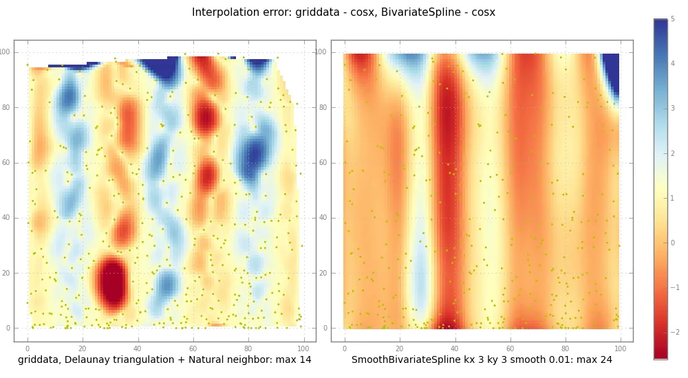
    pl.suptitle( "Interpolation error: griddata - %s, BivariateSpline - %s" % (
        testfunc.__name__, testfunc.__name__ ), fontsize=11 )

    def subplot( z, jplot, label ):
        ax = pl.subplot( 1, nplot, jplot )
        im = pl.imshow(
            np.clip( z, *imclip ),  # plot to same scale
            cmap=pl.cm.RdYlBu,
            interpolation="nearest" )
                # nearest: squares, else imshow interpolates too
                # todo: centre the pixels
        ny, nx = z.shape
        pl.scatter( X*nx, Y*ny, edgecolor="y", s=1 )  # for random XY
        pl.xlabel(label)
        return [ax, im]

    subplot( trierr, 1,
        "griddata, Delaunay triangulation + Natural neighbor: max %.2g" %
        np.nanmax(np.abs(trierr)) )

    ax, im = subplot( splineerr, 2,
        "SmoothBivariateSpline kx %d ky %d smooth %.3g: max %.2g" % (
        kx, ky, smooth, np.nanmax(np.abs(splineerr)) ))

    pl.subplots_adjust( .02, .01, .92, .98, .05, .05 )  # l b r t
    cax = pl.axes([.95, .05, .02, .9])  # l b w h
    pl.colorbar( im, cax=cax )  # -1.5 .. 9 ??
    if plot >= 2:
        pl.savefig( "tmp.png" )
    pl.show() 

关于2D插值，BivariateSpline和griddata的区别。

scipy.interpolate.*BivariateSpline和matplotlib.mlab.griddata 都需要1D数组作为参数：

Znew = griddata( X,Y,Z, Xnew,Ynew )
    # 1d X Y Z Xnew Ynew -> interpolated 2d Znew on meshgrid(Xnew,Ynew)
assert X.ndim == Y.ndim == Z.ndim == 1  and  len(X) == len(Y) == len(Z)

输入的X,Y,Z描述了三维空间中的一个平面或点云： X,Y（或纬度、经度等）是平面上的点，而Z则是它上面的一个表面或地形。 X,Y可能填满大部分矩形[Xmin..Xmax] x [Ymin..Ymax]，也可能只是其中的一个波浪形S或Y。 Z表面可以是光滑的，也可以是光滑加上一些噪声，或者根本不光滑，像粗糙的火山山脉。 Xnew和Ynew通常也是一维的，描述了一个矩形网格，其中有|Xnew| x |Ynew|个点，你想要在这个网格上进行插值或估计Z。
Znew = griddata（...）返回这个网格上的二维数组，np.meshgrid（Xnew，Ynew）：

Znew[Xnew0,Ynew0], Znew[Xnew1,Ynew0], Znew[Xnew2,Ynew0] ...
Znew[Xnew0,Ynew1] ...
Znew[Xnew0,Ynew2] ...
...

当输入的X,Y坐标值与新的Xnew,Ynew坐标值相差较大时，griddata方法会出现问题。

如果任何网格点在输入数据定义的凸包外部（不进行外推），则返回掩码数组。

（“凸包”是由所有X,Y点围成的虚拟橡皮筋所包含的区域。）

griddata方法的工作原理是首先构建输入X,Y的Delaunay三角剖分，然后进行自然邻居插值。这种方法具有鲁棒性和很快的速度。

然而，BivariateSpline方法可以外推，而且会没有警告地生成极端值。此外，Fitpack中的所有*Spline方法都对平滑参数S非常敏感。Dierckx的书（books.google isbn 019853440X p. 89）上写道：
如果S太小，则样条近似过于起伏，并且会捕捉到太多噪声（过拟合）；
如果S太大，则样条将过于平滑并且会丢失信号（欠拟合）。

离散数据的插值很困难，平滑也不容易，而两者同时进行则更加困难。如果XY数据存在大的空洞或非常嘈杂的Z值，那么插值方法应该如何处理呢？（“如果你想卖掉它，你必须对其进行描述。”）

还有更多注意事项：

1维 vs 2维：某些插值方法接受1维或2维的X,Y,Z值。其他插值方法仅接受1维值，因此在插值之前请将其展平：

Xmesh, Ymesh = np.meshgrid( np.linspace(0,1,Nx), np.linspace(0,1,Ny) )
Z = f( Xmesh, Ymesh )  # Nx x Ny
Znew = griddata( Xmesh.flatten(), Ymesh.flatten(), Z.flatten(), Xnew, Ynew )

关于遮罩数组：Matplotlib 可以很好地处理它们，仅绘制未被遮罩/非 NaN 的点。但是我不敢保证一些愚蠢的 NumPy/SciPy 函数能正常工作。检查 X、Y 外凸壳之外的插值，可以像这样：

Znew = griddata(...)
nmask = np.ma.count_masked(Znew)
if nmask > 0:
    print "info: griddata: %d of %d points are masked, not interpolated" % (
        nmask, Znew.size)
    # Znew = Znew.data  # array with NaNs

在极坐标系下： X、Y 和 Xnew、Ynew 应该在同一个空间中，都是直角坐标系，或者都在 [rmin .. rmax] x [tmin .. tmax] 范围内。
要在三维空间中绘制 (r, theta, z) 点：

from mpl_toolkits.mplot3d import Axes3D
Znew = griddata( R,T,Z, Rnew,Tnew )
ax = Axes3D(fig)
ax.plot_surface( Rnew * np.cos(Tnew), Rnew * np.sin(Tnew), Znew )

参见（未尝试）：

ax = subplot(1,1,1, projection="polar", aspect=1.)
ax.pcolormesh(theta, r, Z)

---

对于谨慎的程序员，有两个提示：

检查异常值或奇怪的缩放：

def minavmax( X ):
    m = np.nanmin(X)
    M = np.nanmax(X)
    av = np.mean( X[ - np.isnan(X) ])  # masked ?
    histo = np.histogram( X, bins=5, range=(m,M) ) [0]
    return "min %.2g  av %.2g  max %.2g  histo %s" % (m, av, M, histo)

for nm, x in zip( "X Y Z  Xnew Ynew Znew".split(),
                (X,Y,Z, Xnew,Ynew,Znew) ):
    print nm, minavmax(x)

检查简单数据的插值：

interpolate( X,Y,Z, X,Y )  -- interpolate at the same points
interpolate( X,Y, np.ones(len(X)), Xnew,Ynew )  -- constant 1 ?

- denis