我处理的是基于不规则二维网格的卫星数据,其维度为扫描线(沿轨迹维度)和地面像素(横向维度)。每个中心像素的纬度和经度信息存储在辅助坐标变量中,以及四个角落的坐标对(纬度和经度坐标以WGS84参考椭球体为基准)。数据存储在netCDF4文件中。
我尝试的是在投影地图上高效地绘制这些文件(可能是文件的组合-下一步!)。
到目前为止,我的方法受到Jeremy Voisey对此问题的回答的启发,建立了一个将我感兴趣的变量与像素边界相关联的数据框,并使用
让我说明一下我的工作流程,并提前道歉,因为我的方法很幼稚:我只是在一两周前开始使用R编码。 注意: 为了完全重现问题:
1. 下载两个数据框:so2df.Rda(22M)和pixel_corners.Rda(26M)
2. 将它们加载到您的环境中,例如:
我尝试的是在投影地图上高效地绘制这些文件(可能是文件的组合-下一步!)。
到目前为止,我的方法受到Jeremy Voisey对此问题的回答的启发,建立了一个将我感兴趣的变量与像素边界相关联的数据框,并使用
ggplot2和geom_polygon进行实际绘制。让我说明一下我的工作流程,并提前道歉,因为我的方法很幼稚:我只是在一两周前开始使用R编码。 注意: 为了完全重现问题:
1. 下载两个数据框:so2df.Rda(22M)和pixel_corners.Rda(26M)
2. 将它们加载到您的环境中,例如:
so2df <- readRDS(file="so2df.Rda")
pixel_corners <- readRDS(file="pixel_corners.Rda")
初始设置
我将从文件中读取数据以及纬度/经度边界。
- 跳转到“合并数据框架”步骤。
library(ncdf4)
library(ggplot2)
library(ggmap)
# set path and filename
ncpath <- "/Users/stefano/src/s5p/products/e1dataset/L2__SO2/"
ncname <- "S5P_OFFL_L2__SO2____20171128T234133_20171129T003956_00661_01_022943_00000000T000000"
ncfname <- paste(ncpath, ncname, ".nc", sep="")
nc <- nc_open(ncfname)

# save fill value and multiplication factors
mfactor = ncatt_get(nc, "PRODUCT/sulfurdioxide_total_vertical_column",
                    "multiplication_factor_to_convert_to_DU")
fillvalue = ncatt_get(nc, "PRODUCT/sulfurdioxide_total_vertical_column",
                      "_FillValue")

# read the SO2 total column variable
so2tc <- ncvar_get(nc, "PRODUCT/sulfurdioxide_total_vertical_column")

# read lat/lon of centre pixels
lat <- ncvar_get(nc, "PRODUCT/latitude")
lon <- ncvar_get(nc, "PRODUCT/longitude")

# read latitude and longitude bounds
lat_bounds <- ncvar_get(nc, "GEOLOCATIONS/latitude_bounds")
lon_bounds <- ncvar_get(nc, "GEOLOCATIONS/longitude_bounds")

# close the file
nc_close(nc)
dim(so2tc)
## [1]  450 3244
因此,对于这个文件/密码,每个3244个扫描线都有450个地面像素。
创建数据框
在这里,我创建了两个数据框,一个用于值(经过一些后处理),另一个用于纬度/经度边界,然后将这两个数据框合并。
so2df <- data.frame(lat=as.vector(lat), lon=as.vector(lon), so2tc=as.vector(so2tc))
# add id for each pixel
so2df$id <- row.names(so2df)
# convert to DU
so2df$so2tc <- so2df$so2tc*as.numeric(mfactor$value)
# replace fill values with NA
so2df$so2tc[so2df$so2tc == fillvalue] <- NA
saveRDS(so2df, file="so2df.Rda")
summary(so2df)

##       lat              lon              so2tc              id
##  Min.   :-89.97   Min.   :-180.00   Min.   :-821.33   Length:1459800
##  1st Qu.:-62.29   1st Qu.:-163.30   1st Qu.:  -0.48   Class :character
##  Median :-19.86   Median :-150.46   Median :  -0.08   Mode  :character
##  Mean   :-13.87   Mean   : -90.72   Mean   :  -1.43
##  3rd Qu.: 31.26   3rd Qu.: -27.06   3rd Qu.:   0.26
##  Max.   : 83.37   Max.   : 180.00   Max.   :3015.55
##                                     NA's   :200864
我将这个数据框保存为so2df.Rda 这里(22M)。
num_points = dim(lat_bounds)[1]
pixel_corners <- data.frame(lat_bounds=as.vector(lat_bounds), lon_bounds=as.vector(lon_bounds))
# create id column by replicating pixel's id for each of the 4 corner points
pixel_corners$id <- rep(so2df$id, each=num_points)
saveRDS(pixel_corners, file="pixel_corners.Rda")
summary(pixel_corners)


##    lat_bounds       lon_bounds           id
##  Min.   :-89.96   Min.   :-180.00   Length:5839200
##  1st Qu.:-62.29   1st Qu.:-163.30   Class :character
##  Median :-19.86   Median :-150.46   Mode  :character
##  Mean   :-13.87   Mean   : -90.72
##  3rd Qu.: 31.26   3rd Qu.: -27.06
##  Max.   : 83.40   Max.   : 180.00
如预期,经度/纬度边界数据帧的大小是值数据帧的四倍(每个像素/值有四个点)。
我将此数据帧保存为pixel_corners.Rda在这里(26M)。
合并数据帧
然后我通过id将这两个数据帧合并:
start_time <- Sys.time()
so2df <- merge(pixel_corners, so2df, by=c("id"))
time_taken <- Sys.time() - start_time
print(paste(dim(so2df)[1], "rows merged in", time_taken, "seconds"))

## [1] "5839200 rows merged in 42.4763631820679 seconds"
正如您所看到的,这是一个相当耗费CPU资源的过程。我想知道如果我一次处理15个文件(全局覆盖),会发生什么。
绘制数据
现在,我已经将像素角落与像素值链接起来,可以轻松地绘制它们。通常,我对轨道的特定区域感兴趣,因此我编写了一个在绘制之前对输入数据框进行子集化的函数:
PlotRegion <- function(so2df, latlon, title) {
  # Plot the given dataset over a geographic region.
  #
  # Args:
  #   df: The dataset, should include the no2tc, lat, lon columns
  #   latlon: A vector of four values identifying the botton-left and top-right corners
  #           c(latmin, latmax, lonmin, lonmax)
  #   title: The plot title

  # subset the data frame first
  df_sub <- subset(so2df, lat>latlon[1] & lat<latlon[2] & lon>latlon[3] & lon<latlon[4])

  subtitle = paste("#Pixel =", dim(df_sub)[1], "- Data min =",
                   formatC(min(df_sub$so2tc, na.rm=T), format="e", digits=2), "max =",
                   formatC(max(df_sub$so2tc, na.rm=T), format="e", digits=2))

  ggplot(df_sub) +
    geom_polygon(aes(y=lat_bounds, x=lon_bounds, fill=so2tc, group=id), alpha=0.8) +
    borders('world', xlim=range(df_sub$lon), ylim=range(df_sub$lat),
            colour='gray20', size=.2) +
    theme_light() +
    theme(panel.ontop=TRUE, panel.background=element_blank()) +
    scale_fill_distiller(palette='Spectral') +
    coord_quickmap(xlim=c(latlon[3], latlon[4]), ylim=c(latlon[1], latlon[2])) +
    labs(title=title, subtitle=subtitle,
         x="Longitude", y="Latitude",
         fill=expression(DU))
}
然后我在感兴趣的区域调用我的函数,例如让我们看看在夏威夷发生了什么:
latlon = c(17.5, 22.5, -160, -154)
PlotRegion(so2df, latlon, expression(SO[2]~total~vertical~column))
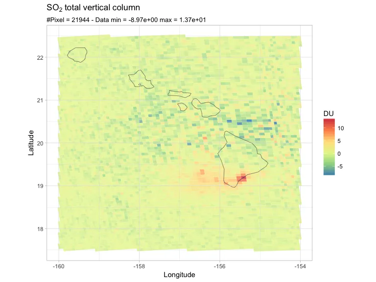
这些是我的像素,似乎来自马乌纳罗亚的SO2烟囱。现在请暂时忽略负值。您可以看到,在观测区域边缘,像素面积会有所变化(采用了不同的分组方案)。
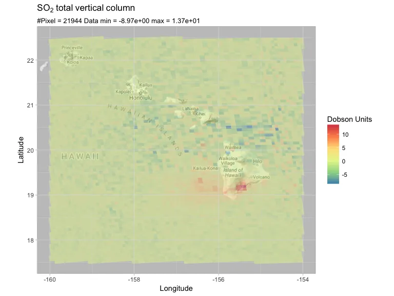
我尝试使用ggmap在谷歌地图上展示相同的图表:
PlotRegionMap <- function(so2df, latlon, title) {
  # Plot the given dataset over a geographic region.
  #
  # Args:
  #   df: The dataset, should include the no2tc, lat, lon columns
  #   latlon: A vector of four values identifying the botton-left and top-right corners
  #           c(latmin, latmax, lonmin, lonmax)
  #   title: The plot title

  # subset the data frame first
  df_sub <- subset(so2df, lat>latlon[1] & lat<latlon[2] & lon>latlon[3] & lon<latlon[4])

  subtitle = paste("#Pixel =", dim(df_sub)[1], "Data min =", formatC(min(df_sub$so2tc, na.rm=T), format="e", digits=2),
                   "max =", formatC(max(df_sub$so2tc, na.rm=T), format="e", digits=2))
  base_map <- get_map(location = c(lon = (latlon[4]+latlon[3])/2, lat = (latlon[1]+latlon[2])/2), zoom = 7, maptype="terrain", color="bw")

  ggmap(base_map, extent = "normal")  +
    geom_polygon(data=df_sub, aes(y=lat_bounds, x=lon_bounds,fill=so2tc, group=id),  alpha=0.5) +
    theme_light() +
    theme(panel.ontop=TRUE, panel.background=element_blank()) +
    scale_fill_distiller(palette='Spectral') +
    coord_quickmap(xlim=c(latlon[3], latlon[4]), ylim=c(latlon[1], latlon[2])) +
    labs(title=title, subtitle=subtitle,
         x="Longitude", y="Latitude",
         fill=expression(DU))

}
这是我得到的内容:
latlon = c(17.5, 22.5, -160, -154)
PlotRegionMap(so2df, latlon, expression(SO[2]~total~vertical~column))
问题
- 有没有更有效的方法来解决这个问题?我正在阅读关于
sf包的内容,想知道是否可以定义一个点数据框(值+中心像素坐标),并让sf自动推断像素边界。这将使我不必依赖于原始数据集中定义的纬度/经度边界,并将它们与我的值合并。我可以接受在扫描的边缘过渡区域上失去精度,因为网格基本上是规则的,每个像素大小为3.5x7 km²。 - 重新对我的数据进行网格化处理(如何?),可能通过聚合相邻像素来提高性能吗?我考虑使用
raster包,据我所知,它需要数据在一个规则的网格上。这应该对全球范围内的绘图有用(例如欧洲地区的绘图),在这种情况下,我不需要绘制单个像素 - 实际上,我甚至看不到它们。 - 在谷歌地图上绘图时,我需要重新投影我的数据吗?
[额外美化问题]
- 有没有更优雅的方法在由其四个角点标识的区域上对我的数据框进行子集操作?
- 我该如何更改颜色比例尺,使高值与低值相比更加突出?我用对数比例尺进行了尝试,但效果不佳。
dput(),或者如果您的数据集太大,请使用模拟数据或内置在您正在使用的软件包中的数据集来重现您的问题),这样其他人就可以运行您的代码。 - Jan Boyerhead()和dput()。不过我会尽快抽出时间来处理这个问题。 - Calum You