如何使用stat_contour完全填充轮廓

Question

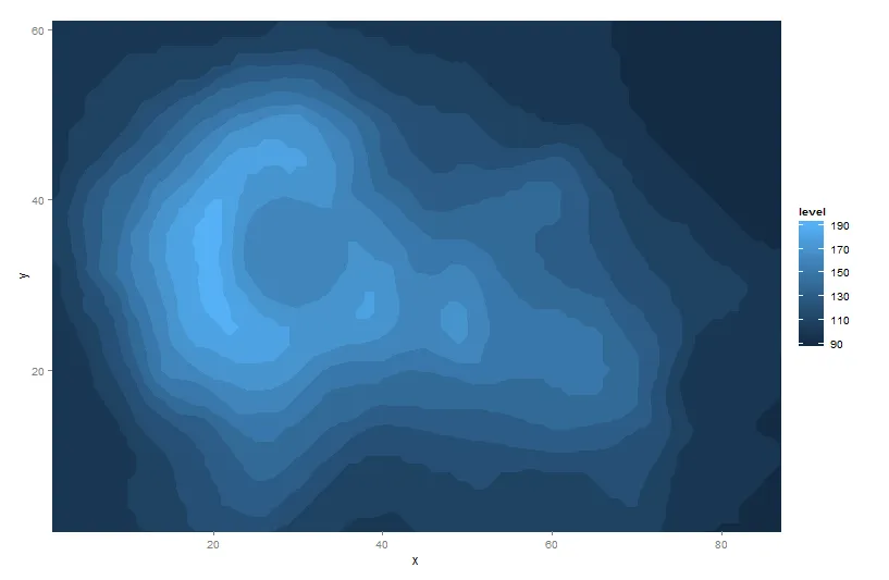
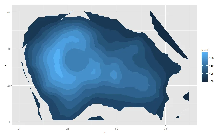
我正在寻找一种方法，可以完全填充由ggplot2的stat_contour生成的轮廓线。当前的结果如下：

# Generate data
library(ggplot2)
library(reshape2) # for melt
volcano3d <- melt(volcano)
names(volcano3d) <- c("x", "y", "z")

v <- ggplot(volcano3d, aes(x, y, z = z))
v + stat_contour(geom="polygon", aes(fill=..level..)) 

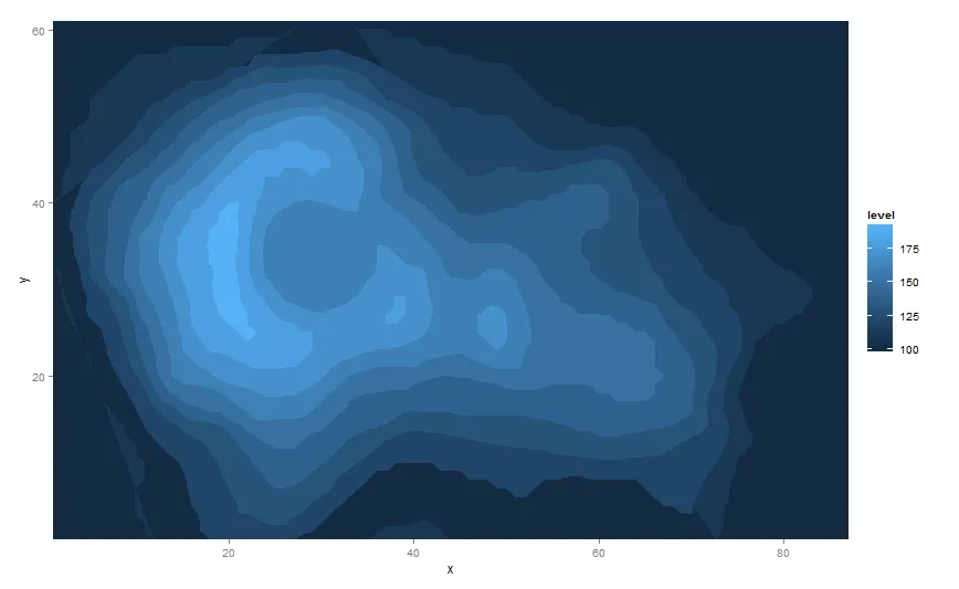
通过手动修改代码，可以获得所需的结果。

v + stat_contour(geom="polygon", aes(fill=..level..)) +
  theme(panel.grid=element_blank())+  # delete grid lines
  scale_x_continuous(limits=c(min(volcano3d$x),max(volcano3d$x)), expand=c(0,0))+ # set x limits
  scale_y_continuous(limits=c(min(volcano3d$y),max(volcano3d$y)), expand=c(0,0))+  # set y limits
  theme(panel.background=element_rect(fill="#132B43"))  # color background

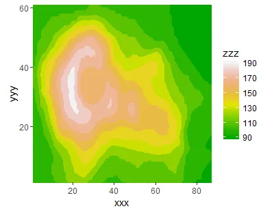
我的问题是，是否有一种方法可以在不手动指定颜色或使用geom_tile()的情况下完全填充绘图?

- chengvt

---

相关：https://dev59.com/soPba4cB1Zd3GeqPqU0w - tonytonov

据我所知，您需要手动扩展数据集。您的解决方案看起来更简单，如果您对其满意，就让它保持原样吧。 - tonytonov

我也看到了那篇文章，但 geom_tile() 使用小矩形，所以不是我要找的效果。filled.contour 到目前为止产生了最好的结果，但它与多个绘图的不兼容性让我尝试使用 ggplots。我想知道是什么产生了透明区域。 - chengvt

你所看到的工件在这里有部分解释：https://dev59.com/U3_aa4cB1Zd3GeqPxgXt。看看能否将该答案适应到你的情况？ - tonytonov

成功了！@tonytonov 非常感谢你！我会在下面发布答案。 - chengvt

Answer 1

正如@tonytonov所建议的那样，在这个线程中，透明区域可以通过闭合多边形来删除。

# check x and y grid
minValue<-sapply(volcano3d,min)
maxValue<-sapply(volcano3d,max)
arbitaryValue=min(volcano3d$z-10)

test1<-data.frame(x=minValue[1]-1,y=minValue[2]:maxValue[2],z=arbitaryValue)
test2<-data.frame(x=minValue[1]:maxValue[1],y=minValue[2]-1,z=arbitaryValue)
test3<-data.frame(x=maxValue[1]+1,y=minValue[2]:maxValue[2],z=arbitaryValue)
test4<-data.frame(x=minValue[1]:maxValue[1],y=maxValue[2]+1,z=arbitaryValue)
test<-rbind(test1,test2,test3,test4)

vol<-rbind(volcano3d,test)

w <- ggplot(vol, aes(x, y, z = z))
w + stat_contour(geom="polygon", aes(fill=..level..)) # better

# Doesn't work when trying to get rid of unwanted space
w + stat_contour(geom="polygon", aes(fill=..level..))+
  scale_x_continuous(limits=c(min(volcano3d$x),max(volcano3d$x)), expand=c(0,0))+ # set x limits
  scale_y_continuous(limits=c(min(volcano3d$y),max(volcano3d$y)), expand=c(0,0))  # set y limits

# work here!
w + stat_contour(geom="polygon", aes(fill=..level..))+
coord_cartesian(xlim=c(min(volcano3d$x),max(volcano3d$x)),
                ylim=c(min(volcano3d$y),max(volcano3d$y)))

这个调整后的问题在于，除了试错法之外，如何找到确定arbitaryValue的方法。

[从这里开始编辑]

这只是一个快速更新，展示我如何在不必为每个数据集猜测的情况下确定arbitaryValue。

BINS<-50
BINWIDTH<-(diff(range(volcano3d$z))/BINS) # reference from ggplot2 code
arbitaryValue=min(volcano3d$z)-BINWIDTH*1.5

这似乎对我目前正在处理的数据集效果很好。不确定是否适用于其他数据集。另外，请注意，我在此处设置BINS值的事实要求我在stat_contour中使用bins=BINS。

- chengvt

---

很高兴能够帮助。不错的解决方案，特别是那些难看的瑕疵现在已经消失了。感谢您的发布！ - tonytonov

Answer 2

感谢@chengvt的回答。我有时需要这种技术，所以我写了一个通用的function()函数。

test_f <- function(df) {
  colname <- names(df)
  names(df) <- c("x", "y", "z")
  Range <- as.data.frame(sapply(df, range))
  Dim <- as.data.frame(t(sapply(df, function(x) length(unique(x)))))
  arb_z = Range$z[1] - diff(Range$z)/20
  df2 <- rbind(df,
               expand.grid(x = c(Range$x[1] - diff(Range$x)/20, Range$x[2] + diff(Range$x)/20), 
                           y = seq(Range$y[1], Range$y[2], length = Dim$y), z = arb_z),
               expand.grid(x = seq(Range$x[1], Range$x[2], length = Dim$x),
                           y = c(Range$y[1] - diff(Range$y)/20, Range$y[2] + diff(Range$y)/20), z = arb_z))
  g <- ggplot(df2, aes(x, y, z = z)) + labs(x = colname[1], y = colname[2], fill = colname[3]) + 
    stat_contour(geom="polygon", aes(fill=..level..)) + 
    coord_cartesian(xlim=c(Range$x), ylim=c(Range$y), expand = F)
  return(g)
}

library(ggplot2); library(reshape2)
volcano3d <- melt(volcano)
names(volcano3d) <- c("xxx", "yyy", "zzz")
test_f(volcano3d) + scale_fill_gradientn(colours = terrain.colors(10))

- cuttlefish44