三元图和填充轮廓。

13

大家好,我希望能够获得有关三元图(“vcd”)的一些提示。

我有这个数据框:

a <- c(0.1, 0.5, 0.5, 0.6, 0.2, 0, 0, 0.004166667, 0.45) 
b <- c(0.75,0.5,0,0.1,0.2,0.951612903,0.918103448,0.7875,0.45)
c <- c(0.15,0,0.5,0.3,0.6,0.048387097,0.081896552,0.208333333,0.1) 
d <- c(500,2324.90,2551.44,1244.50, 551.22,-644.20,-377.17,-100, 2493.04) 
df <- data.frame(a, b, c, d)

我正在构建一个三元图:

ternaryplot(df[,1:3], df$d)

我该如何映射连续变量d,以获得类似于以下结果的输出?

enter image description here


1
欢迎来到StackOverflow。您应该在问题中标记您所编写的语言,或者至少在问题中提及该语言。为此,您可以使用“编辑”按钮。 - ninjagecko
开始使用 RSiteSearch("三元轮廓") 看看是否有帮助?另外,使用 library("sos"); findFn("三元轮廓") - Ben Bolker
谢谢Ben,我也在看这段代码:http://r.789695.n4.nabble.com/Triangular-filled-contour-plot-td1557386.html,但它相当复杂。 - FraNut
我的ggplot2三元扩展中有一个修改过的geom / stat_density2d函数。http://www.ggtern.com。在这里看看:http://ggtern.com/faceting/ - Nicholas Hamilton
5个回答

21

我曾经需要解决一个类似的问题,这部分促使我编写了一个扩展ggplot2的三元图软件包。该软件包可在CRAN上获得。

此问题的输出:enter image description here

构建以上内容的代码:

#Orignal Data as per Question
a <- c(0.1, 0.5,0.5, 0.6, 0.2, 0          , 0         , 0.004166667, 0.45) 
b <- c(0.75,0.5,0  , 0.1, 0.2, 0.951612903,0.918103448, 0.7875     , 0.45)
c <- c(0.15,0  ,0.5, 0.3, 0.6, 0.048387097,0.081896552, 0.208333333, 0.10) 
d <- c(500,2324.90,2551.44,1244.50, 551.22,-644.20,-377.17,-100, 2493.04) 
df <- data.frame(a, b, c, d)

#For labelling each point.
df$id <- 1:nrow(df)

#Build Plot
ggtern(data=df,aes(x=c,y=a,z=b),aes(x,y,z)) + 
  stat_density2d(geom="polygon",
                 n=400,
                 aes(fill=..level..,
                 weight=d,
                 alpha=abs(..level..)),
                 binwidth=100) + 
  geom_density2d(aes(weight=d,color=..level..),
                 n=400,
                 binwidth=100) +
  geom_point(aes(fill=d),color="black",size=5,shape=21) + 
  geom_text(aes(label=id),size=3) + 
  scale_fill_gradient(low="yellow",high="red") + 
  scale_color_gradient(low="yellow",high="red") + 
  theme_tern_rgbw() + 
  theme(legend.justification=c(0,1), legend.position=c(0,1)) + 
  guides(fill = guide_colorbar(order=1),
         alpha= guide_legend(order=2),
         color="none") + 
  labs(  title= "Ternary Plot and Filled Contour",
         fill = "Value, V",alpha="|V - 0|")

#Save Plot
ggsave("TernFilled.png")

@NicholasHamilton 除了两种颜色的渐变,是否可以获得多种颜色的渐变? - Tom Kurushingal
有一种三色渐变色(http://docs.ggplot2.org/current/scale_gradient2.html),您可以指定低、中和高颜色,但我认为超过这个范围会违背Wilkinson的图形语法原则,而这是ggplot2的基本理论(请参见此处http://www.ggtern.com/resources/)。 - Nicholas Hamilton
3
@NicholasHamilton 你好,我正在尝试复制您的示例,但是发现在ggtern中stat_density_2d已被弃用。我尝试了stat_density_tern但无法将权重引入其中。非常感谢任何帮助。谢谢(TIA)。 - Naive_Natural2511

8

这可能不是最优雅的方法,但它能够工作(从头开始,而且没有使用ternaryplot,因为我无法弄清楚如何做到这一点)。

a<- c (0.1, 0.5, 0.5, 0.6, 0.2, 0, 0, 0.004166667, 0.45) 
b<- c (0.75,0.5,0,0.1,0.2,0.951612903,0.918103448,0.7875,0.45)
c<- c (0.15,0,0.5,0.3,0.6,0.048387097,0.081896552,0.208333333,0.1) 
d<- c (500,2324.90,2551.44,1244.50, 551.22,-644.20,-377.17,-100, 2493.04) 
df<- data.frame (a, b, c)


# First create the limit of the ternary plot:
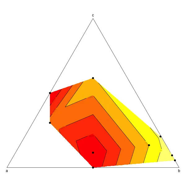
plot(NA,NA,xlim=c(0,1),ylim=c(0,sqrt(3)/2),asp=1,bty="n",axes=F,xlab="",ylab="")
segments(0,0,0.5,sqrt(3)/2)
segments(0.5,sqrt(3)/2,1,0)
segments(1,0,0,0)
text(0.5,(sqrt(3)/2),"c", pos=3)
text(0,0,"a", pos=1)
text(1,0,"b", pos=1)

# The biggest difficulty in the making of a ternary plot is to transform triangular coordinates into cartesian coordinates, here is a small function to do so:
tern2cart <- function(coord){
    coord[1]->x
    coord[2]->y
    coord[3]->z
    x+y+z -> tot
    x/tot -> x  # First normalize the values of x, y and z
    y/tot -> y
    z/tot -> z
    (2*y + z)/(2*(x+y+z)) -> x1 # Then transform into cartesian coordinates
    sqrt(3)*z/(2*(x+y+z)) -> y1
    return(c(x1,y1))
    }

# Apply this equation to each set of coordinates
t(apply(df,1,tern2cart)) -> tern

# Intrapolate the value to create the contour plot
resolution <- 0.001
require(akima)
interp(tern[,1],tern[,2],z=d, xo=seq(0,1,by=resolution), yo=seq(0,1,by=resolution)) -> tern.grid

# And then plot:
image(tern.grid,breaks=c(-1000,0,500,1000,1500,2000,3000),col=rev(heat.colors(6)),add=T)
contour(tern.grid,levels=c(-1000,0,500,1000,1500,2000,3000),add=T)
points(tern,pch=19)

enter image description here


3

我先前的回答使用了密度估计方法。这里是一种使用线性回归的方法。

df <- data.frame(a, b, c, d)
ggtern(df,aes(a,c,b)) + 
  geom_interpolate_tern(aes(value=d,fill=..level..),
                        binwidth=500,
                        colour="white") +
  geom_point(aes(fill=d),color="black",shape=21,size=3) + 
  scale_fill_gradient(low="yellow",high="red") +
  theme(legend.position=c(0,1),legend.justification=c(0,1)) + 
  labs(fill="Value, d")

enter image description here


2
非常感谢您的指引,这是我的最终成果:
#Rename header
names(SI) [6] <- "WATER%"
names(SI) [7] <- "VEGETATION%"
names(SI) [8] <- "SOIL%"

#pdf(file="prova_ternary12.pdf", width = 5, height =5)
##++++++++++++++++++++++++++++++
install.packages("colourschemes", repos="http://R-Forge.R-project.org")
library(colourschemes)
rs = rampInterpolate ( limits =c(-0.8 , 0.8),
                       ramp = c("red4", "red", "orangered", "orange", "darkgoldenrod1", "white", 
                                "cyan2", "blue", "darkblue", "blueviolet", "purple3") )
rs(-0.8)
rs(-0.6000)
rs(-0.4)
rs(-0.2)
rs(0)
rs(0.2)
rs(0.4)
rs(0.6000)
rs(0.8000)


#++++++++++++++++++++++++++++++

#TERNARYPLOT (vcd)
library(vcd)
png(file="ternary.png", width=800, height=800)
 ternaryplot(
  SI[,6:8],
  bg = "lightgray",
  grid_color = "black",
  labels_color = "black",   
  dimnames_position = c("corner"),
  #dimnames = 10,
  newpage = T,
  #dimnames_color = "green",
  border = "black",
  pop=T,
  #SI$MEAN_b2b6.tm,
  col=rs(SI$MEAN_b2b6.TM_V2),
  #col = ifelse(SI$MEAN_b1b6.tm > 0, "blue", "#cd000020"), 
  pch=13, cex=.4, prop_size = F,
  labels = c("outside"),
  #size=SI$MEAN_b1b6.tm,
  main="b4b6  -TM data-")

plotting 3 variables by ternaryplot() and rampInterpulate()


0
我建议使用plotly。这里是一个链接:https://plotly.com/python/ternary-contour/
    import plotly.figure_factory as ff
import numpy as np
Al = np.array([0. , 0. , 0., 0., 1./3, 1./3, 1./3, 2./3, 2./3, 1.])
Cu = np.array([0., 1./3, 2./3, 1., 0., 1./3, 2./3, 0., 1./3, 0.])
Y = 1 - Al - Cu
# synthetic data for mixing enthalpy
# See https://pycalphad.org/docs/latest/examples/TernaryExamples.html
enthalpy = (Al - 0.01) * Cu * (Al - 0.52) * (Cu - 0.48) * (Y - 1)**2
fig = ff.create_ternary_contour(np.array([Al, Y, Cu]), enthalpy,
                                pole_labels=['Al', 'Y', 'Cu'],
                                interp_mode='cartesian')
fig.show()

这里放图片描述


网页内容由stack overflow 提供, 点击上面的
可以查看英文原文,
原文链接