非单调数据（不是一维函数）的三次样条插值法

Question

我有一个如下所示的曲线：

这个图的x坐标和y坐标是：
path_x= (4.0, 5.638304088577984, 6.785456961280076, 5.638304088577984, 4.0)
path_y =(0.0, 1.147152872702092, 2.7854569612800755, 4.423761049858059, 3.2766081771559668)

我通过以下方式获得上述图片：

x_min =min(path_x)-1
x_max =max(path_x)+1
y_min =min(path_y)-1
y_max =max(path_y)+1

num_pts = len(path_x)

fig = plt.figure(figsize=(8,8))
#fig = plt.figure()
plt.suptitle("Curve and the boundary")
ax = fig.add_subplot(1,1,1)

ax.set_xlim([min(x_min,y_min),max(x_max,y_max)])
ax.set_ylim([min(x_min,y_min),max(x_max,y_max)])
ax.plot(path_x,path_y)

现在我的意图是使用三次样条插值法绘制平滑曲线。但是看起来对于三次样条插值，需要使 x 坐标处于升序。而在这种情况下，x 值和 y 值都不是按升序排列的。
同时，这不是一个函数。也就是说，一个 x 值映射到了多个元素的范围内。

我还查阅了这篇帖子。但是我无法找到解决我的问题的合适方法。

我非常感谢您在这方面提供的帮助。

- Charith

---

参数化曲线。您可以将其分解为x(t)和y(t)，这些都是可插值的。 - Mad Physicist

@gune请不要忘记查看我的答案，我将其删除以进行一些修改，然后再次恢复了，因此我担心您没有收到关于我的已更新的答案的通知。 - Arty

你可能会在以下问题中找到一些提示：https://dev59.com/kV4c5IYBdhLWcg3wJnQ- - silgon

Answer 1

如评论所建议，您可以使用任意（且线性！）参数对任何曲线/曲面进行参数化。

例如，定义 t 作为参数，使得您获得 x=x(t) 和 y=y(t)。由于 t 是任意的，您可以定义它，使得在 t=0 时，您获得第一个坐标对 path_x[0],path_y[0]，而在 t=1 时，您获得最后一对坐标 path_x[-1],path_y[-1]。

以下是使用 scipy.interpolate 的代码。

import numpy
import scipy.interpolate
import matplotlib.pyplot as plt

path_x = numpy.asarray((4.0, 5.638304088577984, 6.785456961280076, 5.638304088577984, 4.0),dtype=float)
path_y = numpy.asarray((0.0, 1.147152872702092, 2.7854569612800755, 4.423761049858059, 3.2766081771559668),dtype=float)

# defining arbitrary parameter to parameterize the curve
path_t = numpy.linspace(0,1,path_x.size)

# this is the position vector with
# x coord (1st row) given by path_x, and
# y coord (2nd row) given by path_y
r = numpy.vstack((path_x.reshape((1,path_x.size)),path_y.reshape((1,path_y.size))))

# creating the spline object
spline = scipy.interpolate.interp1d(path_t,r,kind='cubic')

# defining values of the arbitrary parameter over which
# you want to interpolate x and y
# it MUST be within 0 and 1, since you defined
# the spline between path_t=0 and path_t=1
t = numpy.linspace(numpy.min(path_t),numpy.max(path_t),100)

# interpolating along t
# r[0,:] -> interpolated x coordinates
# r[1,:] -> interpolated y coordinates
r = spline(t)

plt.plot(path_x,path_y,'or')
plt.plot(r[0,:],r[1,:],'-k')
plt.xlabel('x')
plt.ylabel('y')
plt.show()

带输出

- Girardi

---

非常感谢您提供带有详细解释的代码！是的，这将起作用。 - Charith

Answer 2

对于非递减的x样条，如果您将x和y函数作为另一个参数t的函数进行计算，则可以轻松地计算出它们：x(t)，y(t)。

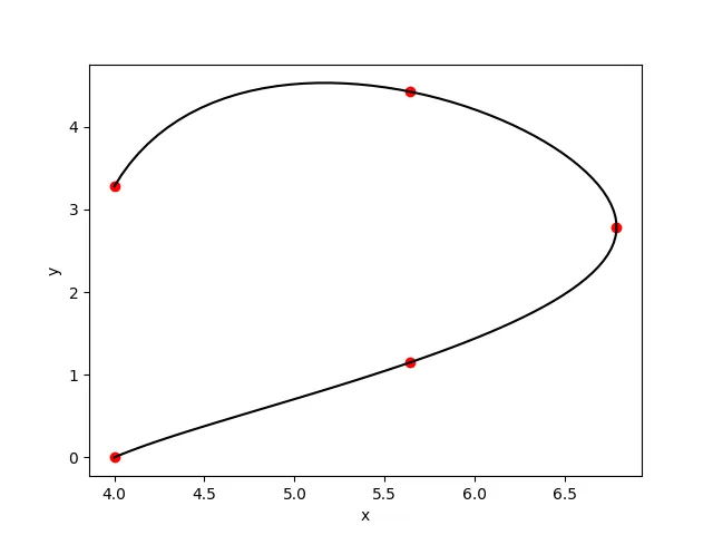
在您的情况下，有5个点，因此t应该是这些点的枚举，即t = 0, 1, 2, 3, 4代表5个点。

所以如果x = [5, 2, 7, 3, 6]，那么x(t) = x(0) = 5，x(1) = 2，x(2) = 7，x(3) = 3，x(4) = 6。同理可得y。

然后为x(t)和y(t)计算样条函数。然后在所有中间的t点计算样条值。最后只需使用所有计算出的值x(t)和y(t)作为函数y(x)的值。

以前，我使用Numpy从头实现了三次样条插值计算，所以如果你不介意的话，我在下面的示例中使用了这段代码（它可能对你学习样条数学有用），请用你的库函数替换。此外，在我的代码中，你可以看到已经注释掉了numba行，如果你想的话，可以使用这些Numba注释来加速计算。

你需要查看代码底部的main()函数，它展示了如何计算和使用x(t)和y(t)。

在线试玩！

import numpy as np, matplotlib.pyplot as plt

# Solves linear system given by Tridiagonal Matrix
# Helper for calculating cubic splines
#@numba.njit(cache = True, fastmath = True, inline = 'always')
def tri_diag_solve(A, B, C, F):
    n = B.size
    assert A.ndim == B.ndim == C.ndim == F.ndim == 1 and (
        A.size == B.size == C.size == F.size == n
    ) #, (A.shape, B.shape, C.shape, F.shape)
    Bs, Fs = np.zeros_like(B), np.zeros_like(F)
    Bs[0], Fs[0] = B[0], F[0]
    for i in range(1, n):
        Bs[i] = B[i] - A[i] / Bs[i - 1] * C[i - 1]
        Fs[i] = F[i] - A[i] / Bs[i - 1] * Fs[i - 1]
    x = np.zeros_like(B)
    x[-1] = Fs[-1] / Bs[-1]
    for i in range(n - 2, -1, -1):
        x[i] = (Fs[i] - C[i] * x[i + 1]) / Bs[i]
    return x
    
# Calculate cubic spline params
#@numba.njit(cache = True, fastmath = True, inline = 'always')
def calc_spline_params(x, y):
    a = y
    h = np.diff(x)
    c = np.concatenate((np.zeros((1,), dtype = y.dtype),
        np.append(tri_diag_solve(h[:-1], (h[:-1] + h[1:]) * 2, h[1:],
        ((a[2:] - a[1:-1]) / h[1:] - (a[1:-1] - a[:-2]) / h[:-1]) * 3), 0)))
    d = np.diff(c) / (3 * h)
    b = (a[1:] - a[:-1]) / h + (2 * c[1:] + c[:-1]) / 3 * h
    return a[1:], b, c[1:], d

# Spline value calculating function, given params and "x"
#@numba.njit(cache = True, fastmath = True, inline = 'always')
def func_spline(x, ix, x0, a, b, c, d):
    dx = x - x0[1:][ix]
    return a[ix] + (b[ix] + (c[ix] + d[ix] * dx) * dx) * dx

# Compute piece-wise spline function for "x" out of sorted "x0" points
#@numba.njit([f'f{ii}[:](f{ii}[:], f{ii}[:], f{ii}[:], f{ii}[:], f{ii}[:], f{ii}[:])' for ii in (4, 8)],
#    cache = True, fastmath = True, inline = 'always')
def piece_wise_spline(x, x0, a, b, c, d):
    xsh = x.shape
    x = x.ravel()
    ix = np.searchsorted(x0[1 : -1], x)
    y = func_spline(x, ix, x0, a, b, c, d)
    y = y.reshape(xsh)
    return y

def main():
    x0 = np.array([4.0, 5.638304088577984, 6.785456961280076, 5.638304088577984, 4.0])
    y0 = np.array([0.0, 1.147152872702092, 2.7854569612800755, 4.423761049858059, 3.2766081771559668])
    t0 = np.arange(len(x0)).astype(np.float64)
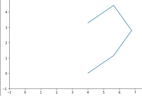
    plt.plot(x0, y0)
    vs = []
    for e in (x0, y0):
        a, b, c, d = calc_spline_params(t0, e)
        x = np.linspace(0, t0[-1], 100)
        vs.append(piece_wise_spline(x, t0, a, b, c, d))
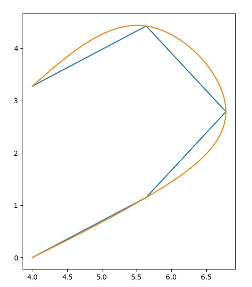
    plt.plot(vs[0], vs[1])
    plt.show()

if __name__ == '__main__':
    main()

输出：

- Arty