我有两个列表来描述函数 y(x):
x = [0,1,2,3,4,5]
y = [12,14,22,39,58,77]
我希望能进行三次样条插值,以便在给定定义域x内的某些值u的情况下使用。
u = 1.25
我可以找到y(u)。
我在SciPy中找到了这个,但是我不确定如何使用它。
我有两个列表来描述函数 y(x):
x = [0,1,2,3,4,5]
y = [12,14,22,39,58,77]
我希望能进行三次样条插值,以便在给定定义域x内的某些值u的情况下使用。
u = 1.25
我可以找到y(u)。
我在SciPy中找到了这个,但是我不确定如何使用它。
简短回答:
from scipy import interpolate

def f(x):
    x_points = [ 0, 1, 2, 3, 4, 5]
    y_points = [12,14,22,39,58,77]

    tck = interpolate.splrep(x_points, y_points)
    return interpolate.splev(x, tck)

print(f(1.25))
长篇回答:
scipy将样条插值步骤分为两个操作,很可能是出于计算效率的考虑。
使用splrep()计算描述样条曲线的系数。splrep返回一个包含系数的元组数组。
这些系数被传递给splev(),以在所需点x(在本例中为1.25)处实际评估样条。
x也可以是一个数组。调用f([1.0, 1.25, 1.5])分别返回1、1.25和1.5处的插值点。
这种方法对于单次评估确实不方便,但由于最常见的用例是从一些函数评估点开始,然后重复使用样条来查找插值值,在实践中通常非常有用。
如果未安装scipy:
import numpy as np
from math import sqrt

def cubic_interp1d(x0, x, y):
    """
    Interpolate a 1-D function using cubic splines.
      x0 : a float or an 1d-array
      x : (N,) array_like
          A 1-D array of real/complex values.
      y : (N,) array_like
          A 1-D array of real values. The length of y along the
          interpolation axis must be equal to the length of x.

    Implement a trick to generate at first step the cholesky matrice L of
    the tridiagonal matrice A (thus L is a bidiagonal matrice that
    can be solved in two distinct loops).

    additional ref: www.math.uh.edu/~jingqiu/math4364/spline.pdf
    """
    x = np.asfarray(x)
    y = np.asfarray(y)

    # remove non finite values
    # indexes = np.isfinite(x)
    # x = x[indexes]
    # y = y[indexes]

    # check if sorted
    if np.any(np.diff(x) < 0):
        indexes = np.argsort(x)
        x = x[indexes]
        y = y[indexes]

    size = len(x)

    xdiff = np.diff(x)
    ydiff = np.diff(y)

    # allocate buffer matrices
    Li = np.empty(size)
    Li_1 = np.empty(size-1)
    z = np.empty(size)

    # fill diagonals Li and Li-1 and solve [L][y] = [B]
    Li[0] = sqrt(2*xdiff[0])
    Li_1[0] = 0.0
    B0 = 0.0 # natural boundary
    z[0] = B0 / Li[0]

    for i in range(1, size-1, 1):
        Li_1[i] = xdiff[i-1] / Li[i-1]
        Li[i] = sqrt(2*(xdiff[i-1]+xdiff[i]) - Li_1[i-1] * Li_1[i-1])
        Bi = 6*(ydiff[i]/xdiff[i] - ydiff[i-1]/xdiff[i-1])
        z[i] = (Bi - Li_1[i-1]*z[i-1])/Li[i]

    i = size - 1
    Li_1[i-1] = xdiff[-1] / Li[i-1]
    Li[i] = sqrt(2*xdiff[-1] - Li_1[i-1] * Li_1[i-1])
    Bi = 0.0 # natural boundary
    z[i] = (Bi - Li_1[i-1]*z[i-1])/Li[i]

    # solve [L.T][x] = [y]
    i = size-1
    z[i] = z[i] / Li[i]
    for i in range(size-2, -1, -1):
        z[i] = (z[i] - Li_1[i-1]*z[i+1])/Li[i]

    # find index
    index = x.searchsorted(x0)
    np.clip(index, 1, size-1, index)

    xi1, xi0 = x[index], x[index-1]
    yi1, yi0 = y[index], y[index-1]
    zi1, zi0 = z[index], z[index-1]
    hi1 = xi1 - xi0

    # calculate cubic
    f0 = zi0/(6*hi1)*(xi1-x0)**3 + \
         zi1/(6*hi1)*(x0-xi0)**3 + \
         (yi1/hi1 - zi1*hi1/6)*(x0-xi0) + \
         (yi0/hi1 - zi0*hi1/6)*(xi1-x0)
    return f0

if __name__ == '__main__':
    import matplotlib.pyplot as plt
    x = np.linspace(0, 10, 11)
    y = np.sin(x)
    plt.scatter(x, y)

    x_new = np.linspace(0, 10, 201)
    plt.plot(x_new, cubic_interp1d(x_new, x, y))

    plt.show()
x = [-8,-4.19,-3.54,-3.31,-2.56,-2.31,-1.66,-0.96,-0.22,0.62,1.21,3] y = [-0.01,0.01,0.03,0.04,0.07,0.09,0.16,0.28,0.45,0.65,0.77,1],那么它无法正常工作。如果您在 x 数组中将 -8 更改为 -5,则可以正常工作。 - palloc#!/usr/bin/env python3
import scipy
scipy.version.version
如果您的scipy版本大于等于0.18.0,则可以运行以下示例代码进行三次样条插值:
#!/usr/bin/env python3

import numpy as np
from scipy.interpolate import CubicSpline

# calculate 5 natural cubic spline polynomials for 6 points
# (x,y) = (0,12) (1,14) (2,22) (3,39) (4,58) (5,77)
x = np.array([0, 1, 2, 3, 4, 5])
y = np.array([12,14,22,39,58,77])

# calculate natural cubic spline polynomials
cs = CubicSpline(x,y,bc_type='natural')

# show values of interpolation function at x=1.25
print('S(1.25) = ', cs(1.25))

## Aditional - find polynomial coefficients for different x regions

# if you want to print polynomial coefficients in form
# S0(0<=x<=1) = a0 + b0(x-x0) + c0(x-x0)^2 + d0(x-x0)^3
# S1(1< x<=2) = a1 + b1(x-x1) + c1(x-x1)^2 + d1(x-x1)^3
# ...
# S4(4< x<=5) = a4 + b4(x-x4) + c5(x-x4)^2 + d5(x-x4)^3
# x0 = 0; x1 = 1; x4 = 4; (start of x region interval)

# show values of a0, b0, c0, d0, a1, b1, c1, d1 ...
cs.c

# Polynomial coefficients for 0 <= x <= 1
a0 = cs.c.item(3,0)
b0 = cs.c.item(2,0)
c0 = cs.c.item(1,0)
d0 = cs.c.item(0,0)

# Polynomial coefficients for 1 < x <= 2
a1 = cs.c.item(3,1)
b1 = cs.c.item(2,1)
c1 = cs.c.item(1,1)
d1 = cs.c.item(0,1)

# ...

# Polynomial coefficients for 4 < x <= 5
a4 = cs.c.item(3,4)
b4 = cs.c.item(2,4)
c4 = cs.c.item(1,4)
d4 = cs.c.item(0,4)

# Print polynomial equations for different x regions
print('S0(0<=x<=1) = ', a0, ' + ', b0, '(x-0) + ', c0, '(x-0)^2  + ', d0, '(x-0)^3')
print('S1(1< x<=2) = ', a1, ' + ', b1, '(x-1) + ', c1, '(x-1)^2  + ', d1, '(x-1)^3')
print('...')
print('S5(4< x<=5) = ', a4, ' + ', b4, '(x-4) + ', c4, '(x-4)^2  + ', d4, '(x-4)^3')

# So we can calculate S(1.25) by using equation S1(1< x<=2)
print('S(1.25) = ', a1 + b1*0.25 + c1*(0.25**2) + d1*(0.25**3))

# Cubic spline interpolation calculus example
    #  https://www.youtube.com/watch?v=gT7F3TWihvk
|bi| > |ai| + |ci|,其中ai = h[i],bi = 2*(h[i]+h[i+1]),ci = h[i+1],其中h[i]无条件为正数。(参见https://www.cfd-online.com/Wiki/Tridiagonal_matrix_algorithm_-TDMA(Thomas_algorithm))
我再次提到来自jingqiu的文档(请参阅我的先前帖子,不幸的是链接已经失效,但仍然可以在Web缓存中找到它)。
TDMA求解器的优化版本可以描述如下:
def TDMAsolver(a,b,c,d):
""" This function is licenced under: Attribution-ShareAlike 3.0 Unported (CC BY-SA 3.0)
    https://creativecommons.org/licenses/by-sa/3.0/
    Author raphael valentin
    Date 25 Mar 2022
    ref. https://www.cfd-online.com/Wiki/Tridiagonal_matrix_algorithm_-_TDMA_(Thomas_algorithm)
"""
n = len(d)

w = np.empty(n-1,float)
g = np.empty(n, float)

w[0] = c[0]/b[0]
g[0] = d[0]/b[0]

for i in range(1, n-1):
    m = b[i] - a[i-1]*w[i-1]
    w[i] = c[i] / m
    g[i] = (d[i] - a[i-1]*g[i-1]) / m
g[n-1] = (d[n-1] - a[n-2]*g[n-2]) / (b[n-1] - a[n-2]*w[n-2])

for i in range(n-2, -1, -1):
    g[i] = g[i] - w[i]*g[i+1]

return g
当我们可以获取每个个体的 ai, bi, ci, di 时,将这些定义组合到自然三次样条插值器函数中就变得容易了,只需在这两个循环内完成。
def cubic_interpolate(x0, x, y):
""" Natural cubic spline interpolate function
    This function is licenced under: Attribution-ShareAlike 3.0 Unported (CC BY-SA 3.0)
    https://creativecommons.org/licenses/by-sa/3.0/
    Author raphael valentin
    Date 25 Mar 2022
"""
xdiff = np.diff(x)
dydx = np.diff(y)
dydx /= xdiff

n = size = len(x)

w = np.empty(n-1, float)
z = np.empty(n, float)

w[0] = 0.
z[0] = 0.
for i in range(1, n-1):
    m = xdiff[i-1] * (2 - w[i-1]) + 2 * xdiff[i]
    w[i] = xdiff[i] / m
    z[i] = (6*(dydx[i] - dydx[i-1]) - xdiff[i-1]*z[i-1]) / m
z[-1] = 0.

for i in range(n-2, -1, -1):
    z[i] = z[i] - w[i]*z[i+1]

# find index (it requires x0 is already sorted)
index = x.searchsorted(x0)
np.clip(index, 1, size-1, index)

xi1, xi0 = x[index], x[index-1]
yi1, yi0 = y[index], y[index-1]
zi1, zi0 = z[index], z[index-1]
hi1 = xi1 - xi0

# calculate cubic
f0 = zi0/(6*hi1)*(xi1-x0)**3 + \
    zi1/(6*hi1)*(x0-xi0)**3 + \
    (yi1/hi1 - zi1*hi1/6)*(x0-xi0) + \
    (yi0/hi1 - zi0*hi1/6)*(xi1-x0)
return f0
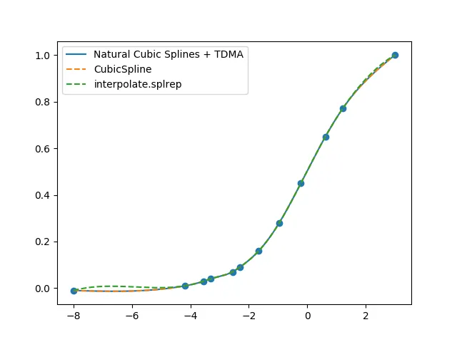
scipy.interpolate中的CubicSpline函数/类相同,如下图所示。
 还可以实现第一和第二阶解析导数,可以描述为:
f1p = -zi0/(2*hi1)*(xi1-x0)**2 + zi1/(2*hi1)*(x0-xi0)**2 + (yi1/hi1 - zi1*hi1/6) + (yi0/hi1 - zi0*hi1/6)
f2p = zi0/hi1 * (xi1-x0) + zi1/hi1 * (x0-xi0)
那么,很容易验证f2p[0]和f2p[-1]等于0,然后插值函数会产生自然样条。
关于自然样条的额外参考资料: https://faculty.ksu.edu.sa/sites/default/files/numerical_analysis_9th.pdf#page=167
一个使用示例:
import matplotlib.pyplot as plt
import numpy as np
x = [-8,-4.19,-3.54,-3.31,-2.56,-2.31,-1.66,-0.96,-0.22,0.62,1.21,3]
y = [-0.01,0.01,0.03,0.04,0.07,0.09,0.16,0.28,0.45,0.65,0.77,1]
x = np.asfarray(x)
y = np.asfarray(y)

plt.scatter(x, y)
x_new= np.linspace(min(x), max(x), 10000)
y_new = cubic_interpolate(x_new, x, y)
plt.plot(x_new, y_new)

from scipy.interpolate import CubicSpline
f = CubicSpline(x, y, bc_type='natural')
plt.plot(x_new, f(x_new), label='ref')
plt.legend()
plt.show()
如果您想要一个无需依赖的解决方案,可以将以下代码放在这里。
代码取自上面的答案:https://dev59.com/1FwZ5IYBdhLWcg3wWvRY#48085583
def my_cubic_interp1d(x0, x, y):
    """
    Interpolate a 1-D function using cubic splines.
      x0 : a 1d-array of floats to interpolate at
      x : a 1-D array of floats sorted in increasing order
      y : A 1-D array of floats. The length of y along the
          interpolation axis must be equal to the length of x.

    Implement a trick to generate at first step the cholesky matrice L of
    the tridiagonal matrice A (thus L is a bidiagonal matrice that
    can be solved in two distinct loops).

    additional ref: www.math.uh.edu/~jingqiu/math4364/spline.pdf
    # original function code at: https://dev59.com/1FwZ5IYBdhLWcg3wWvRY#48085583


    This function is licenced under: Attribution-ShareAlike 3.0 Unported (CC BY-SA 3.0)
    https://creativecommons.org/licenses/by-sa/3.0/
    Original Author raphael valentin
    Date 3 Jan 2018


    Modifications made to remove numpy dependencies:
        -all sub-functions by MR

    This function, and all sub-functions, are licenced under: Attribution-ShareAlike 3.0 Unported (CC BY-SA 3.0)

    Mod author: Matthew Rowles
    Date 3 May 2021

    """
    def diff(lst):
        """
        numpy.diff with default settings
        """
        size = len(lst)-1
        r = [0]*size
        for i in range(size):
            r[i] = lst[i+1] - lst[i]
        return r

    def list_searchsorted(listToInsert, insertInto):
        """
        numpy.searchsorted with default settings
        """
        def float_searchsorted(floatToInsert, insertInto):
            for i in range(len(insertInto)):
                if floatToInsert <= insertInto[i]:
                    return i
            return len(insertInto)
        return [float_searchsorted(i, insertInto) for i in listToInsert]

    def clip(lst, min_val, max_val, inPlace = False):
        """
        numpy.clip
        """
        if not inPlace:
            lst = lst[:]
        for i in range(len(lst)):
            if lst[i] < min_val:
                lst[i] = min_val
            elif lst[i] > max_val:
                lst[i] = max_val
        return lst

    def subtract(a,b):
        """
        returns a - b
        """
        return a - b

    size = len(x)

    xdiff = diff(x)
    ydiff = diff(y)

    # allocate buffer matrices
    Li   = [0]*size
    Li_1 = [0]*(size-1)
    z    = [0]*(size)

    # fill diagonals Li and Li-1 and solve [L][y] = [B]
    Li[0]   = sqrt(2*xdiff[0])
    Li_1[0] = 0.0
    B0      = 0.0 # natural boundary
    z[0]    = B0 / Li[0]

    for i in range(1, size-1, 1):
        Li_1[i] = xdiff[i-1] / Li[i-1]
        Li[i] = sqrt(2*(xdiff[i-1]+xdiff[i]) - Li_1[i-1] * Li_1[i-1])
        Bi = 6*(ydiff[i]/xdiff[i] - ydiff[i-1]/xdiff[i-1])
        z[i] = (Bi - Li_1[i-1]*z[i-1])/Li[i]

    i = size - 1
    Li_1[i-1] = xdiff[-1] / Li[i-1]
    Li[i]     = sqrt(2*xdiff[-1] - Li_1[i-1] * Li_1[i-1])
    Bi        = 0.0 # natural boundary
    z[i]      = (Bi - Li_1[i-1]*z[i-1])/Li[i]

    # solve [L.T][x] = [y]
    i = size-1
    z[i] = z[i] / Li[i]
    for i in range(size-2, -1, -1):
        z[i] = (z[i] - Li_1[i-1]*z[i+1])/Li[i]

    # find index
    index = list_searchsorted(x0,x)
    index = clip(index, 1, size-1)

    xi1 = [x[num]   for num in index]
    xi0 = [x[num-1] for num in index]
    yi1 = [y[num]   for num in index]
    yi0 = [y[num-1] for num in index]
    zi1 = [z[num]   for num in index]
    zi0 = [z[num-1] for num in index]
    hi1 = list( map(subtract, xi1, xi0) )

    # calculate cubic - all element-wise multiplication
    f0 = [0]*len(hi1)
    for j in range(len(f0)):
        f0[j] = zi0[j]/(6*hi1[j])*(xi1[j]-x0[j])**3 + \
                zi1[j]/(6*hi1[j])*(x0[j]-xi0[j])**3 + \
                (yi1[j]/hi1[j] - zi1[j]*hi1[j]/6)*(x0[j]-xi0[j]) + \
                (yi0[j]/hi1[j] - zi0[j]*hi1[j]/6)*(xi1[j]-x0[j])

    return f0
如果您想获取数值
from scipy.interpolate import CubicSpline
import numpy as np

x = [-5,-4.19,-3.54,-3.31,-2.56,-2.31,-1.66,-0.96,-0.22,0.62,1.21,3]
y = [-0.01,0.01,0.03,0.04,0.07,0.09,0.16,0.28,0.45,0.65,0.77,1]
value = 2

#ascending order
if np.any(np.diff(x) < 0):
    indexes = np.argsort(x).astype(int)
    x = np.array(x)[indexes]
    y = np.array(y)[indexes]

f = CubicSpline(x, y, bc_type='natural')
specificVal = f(value).item(0) #f(value) is numpy.ndarray!!
print(specificVal)
np.linspace的第三个参数可以增加“精度”。from scipy.interpolate import CubicSpline
import numpy as np
import matplotlib.pyplot as plt
x = [-5,-4.19,-3.54,-3.31,-2.56,-2.31,-1.66,-0.96,-0.22,0.62,1.21,3]
y = [-0.01,0.01,0.03,0.04,0.07,0.09,0.16,0.28,0.45,0.65,0.77,1]
#ascending order
if np.any(np.diff(x) < 0):
indexes = np.argsort(x).astype(int)
x = np.array(x)[indexes]
y = np.array(y)[indexes]
f = CubicSpline(x, y, bc_type='natural')
x_new = np.linspace(min(x), max(x), 100)
y_new = f(x_new)
plt.plot(x_new, y_new)
plt.scatter(x, y)
plt.title('Cubic Spline Interpolation')
plt.show()
输出:

最简单的Python3代码:
from scipy import interpolate

if __name__ == '__main__':
    x = [ 0, 1, 2, 3, 4, 5]
    y = [12,14,22,39,58,77]

    # tck : tuple (t,c,k) a tuple containing the vector of knots,
    # the B-spline coefficients, and the degree of the spline.
    tck = interpolate.splrep(x, y)

    print(interpolate.splev(1.25, tck)) # Prints 15.203125000000002
    print(interpolate.splev(...other_value_here..., tck))
根据cwhy的评论和youngmit的回答
是的,正如其他人已经指出的那样,它应该很简单。
>>> from scipy.interpolate import CubicSpline

>>> CubicSpline(x,y)(u)
array(15.203125)
(例如,您可以将其转换为浮点数以从0d NumPy数组中获取值)
尚未描述的是边界条件:如果您对要插值的数据没有任何了解,则默认的“非结节”边界条件效果最佳。
如果您在图中看到以下“特征”,则可以微调边界条件以获得更好的结果:
bc_type='clamped'bc_type='natural'bc_type='periodic'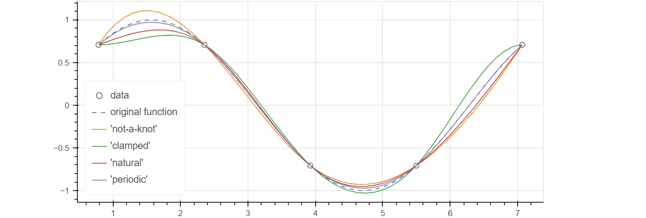
请查看我的文章,了解更多细节和交互式演示。
tck = interpolate.splrep(x_points, y_points)和其上面的两行代码移到f(x)函数外部来避免每次调用函数时计算样条插值。 - cwhynp未被使用。 - Christophe Roussytck,请参考https://docs.scipy.org/doc/scipy/reference/generated/scipy.interpolate.splrep.html#scipy.interpolate.splrep - icemtelprint(interpolate.splev(1.25, tck));-) - AstroFloyd