绘制标量场

Question

我正在寻找一种以标量场的形式绘制此函数的方法，特别是以连续的标量场形式：

library(rgl)

points = seq(-2, 0, length=20)

XY = expand.grid(X=points,Y=-points)
Zf <- function(X,Y){
     X^2-Y^2;
     }
Z <- Zf(XY$X, XY$Y)

open3d()
rgl.surface(x=points, y=matrix(Z,20), coords=c(1,3,2),z=-points)
axes3d()

标量场通常用两个轴X和Y绘制，其中Z由颜色表示(http://en.wikipedia.org/wiki/Scalar_field)

使用ggplot()可以实现这个功能:

daf=data.frame(XY$X,XY$Y,Z)

ggplot(daf)+geom_point(aes(XY.X,XY.Y,color=Z))

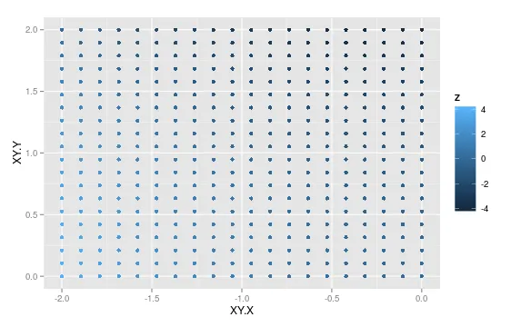
但仍然不是一个连续的领域。

- user3083324

---

你能否更具体/明确地说明你想要的是什么？你的代码没有做到什么？ - Ben Bolker

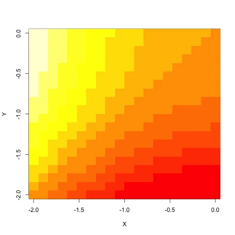
你只需要使用 geom_tile 吗？ggplot(daf)+geom_tile(aes(XY.X,XY.Y,fill=Z)) - MrFlick

不太像 geom_tile，它只是使用矩形而不是点。 - user3083324

Answer 1

这可以通过'image'函数实现：

Z <- outer(points, points, Zf)
image(points, points, Z)

这种方法只使用最近邻插值，但如果您想要更平滑的表示，可以使用其他类型的插值：

library(fields)

# Bilinear interpolation
interp_points = seq(-2, 0, length = 200)
interp_bilinear <- interp.surface(list(x = X, y = Y, z = Z), 
                                  loc = expand.grid(interp_points, interp_points))

image(interp_points, interp_points, matrix(interp_bilinear, 200, 200))

# Bicubic interpolation
library(akima)
interp_bicubic <- bicubic.grid(X, Y, Z, xlim = c(-2, 0), ylim = c(-2, 0), 
                               dx = 2 / (200 - 1), dy = 2 / (200 - 1))
image(interp_bicubic)

不同插值方案的差异在观测数据较少或函数行为更加奇异时变得更加明显：

- Lars Lau Raket