Python绘制多标签分类混淆矩阵的图表

Question

我正在寻找能帮我绘制混淆矩阵的人。我需要这个东西写学术论文。但是我对编程几乎没有经验。

在图片中，你可以看到我的分类报告和我的y_test和X_test的结构，在我的情况下，它们是dtree_predictions。

如果有人能帮我就太好了，因为我已经尝试了很多方法，但是我只得到了错误信息。

X_train, X_test, y_train, y_test = train_test_split(X, Y_profile, test_size = 0.3, random_state = 30)

dtree_model = DecisionTreeClassifier().fit(X_train,y_train)
dtree_predictions = dtree_model.predict(X_test)

print(metrics.classification_report(dtree_predictions, y_test))
              precision    recall  f1-score   support

       0       1.00      1.00      1.00       222
       1       1.00      1.00      1.00       211
       2       1.00      1.00      1.00       229
       3       0.96      0.97      0.96       348
       4       0.89      0.85      0.87        93
       5       0.86      0.86      0.86       105
       6       0.94      0.93      0.94       116
       7       1.00      1.00      1.00       364
       8       0.99      0.97      0.98       139
       9       0.98      0.99      0.99       159
      10       0.97      0.96      0.97       189
      11       0.92      0.92      0.92       124
      12       0.92      0.92      0.92       119
      13       0.95      0.96      0.95       230
      14       0.98      0.96      0.97       452
      15       0.91      0.96      0.93       210

micro avg       0.96      0.96      0.96      3310
macro avg       0.95      0.95      0.95      3310
weighted avg    0.97      0.96      0.96      3310
samples avg     0.96      0.96      0.96      3310

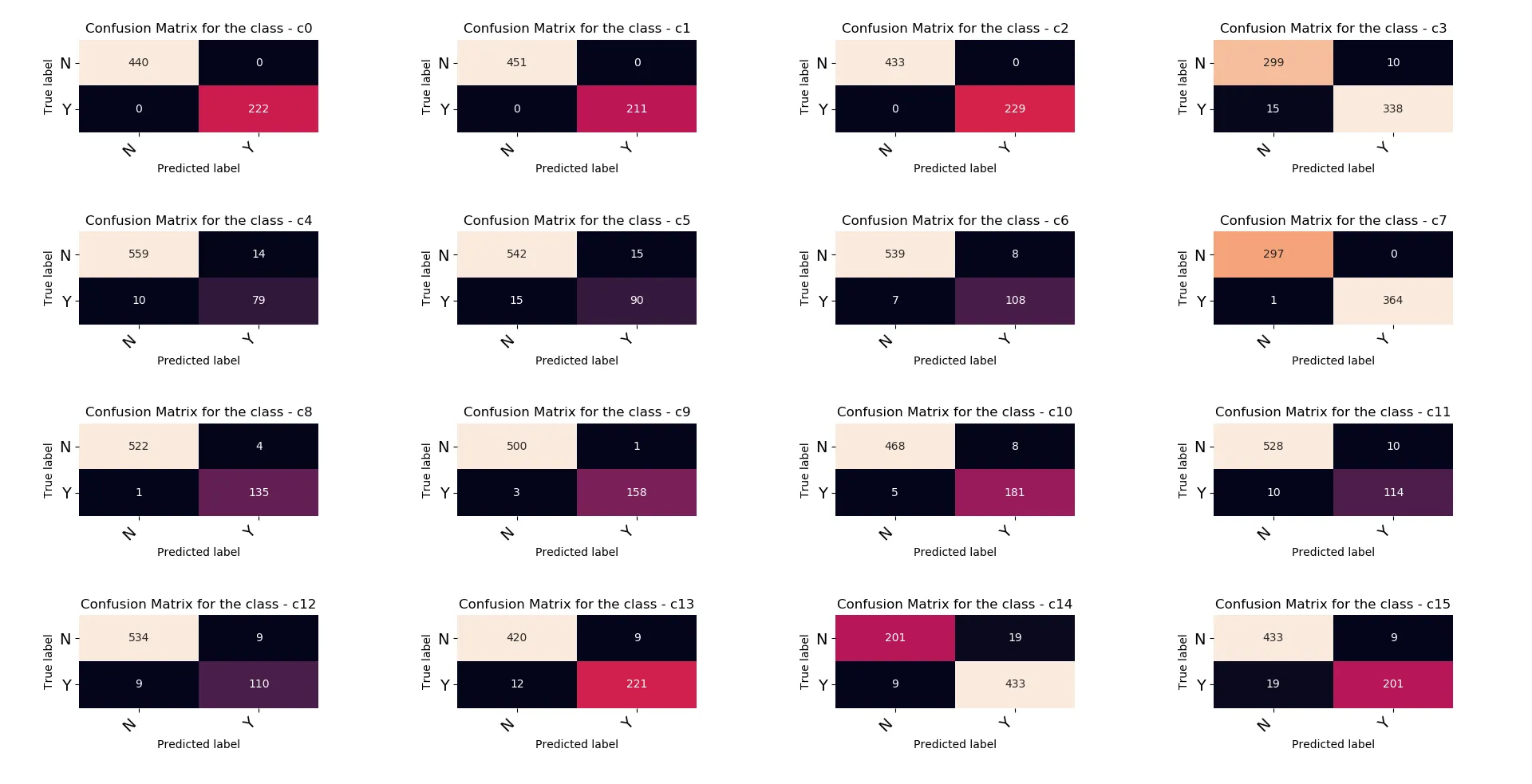
接下来我将打印多标签混淆矩阵的度量

from sklearn.metrics import multilabel_confusion_matrix
multilabel_confusion_matrix(y_test, dtree_predictions)

array([[[440,   0],
    [  0, 222]],

   [[451,   0],
    [  0, 211]],

   [[433,   0],
    [  0, 229]],

   [[299,  10],
    [ 15, 338]],

   [[559,  14],
    [ 10,  79]],

   [[542,  15],
    [ 15,  90]],

   [[539,   8],
    [  7, 108]],

   [[297,   0],
    [  1, 364]],

   [[522,   4],
    [  1, 135]],

   [[500,   1],
    [  3, 158]],

   [[468,   8],
    [  5, 181]],

   [[528,  10],
    [ 10, 114]],

   [[534,   9],
    [  9, 110]],

   [[420,   9],
    [ 12, 221]],

   [[201,  19],
    [  9, 433]],

   [[433,   9],
    [ 19, 201]]])

关于y_test和dtree_predictons的结构。

print(dtree_predictions)
print(dtree_predictions.shape)

[[0. 0. 1. ... 0. 1. 0.]
[1. 0. 0. ... 0. 1. 0.]
[0. 0. 1. ... 0. 1. 0.]
 ...
[1. 0. 0. ... 0. 0. 1.]
[0. 1. 0. ... 1. 0. 1.]
[0. 1. 0. ... 1. 0. 1.]]
(662, 16)

print(y_test)

      Cooler close to failure  Cooler reduced effiency  Cooler full    effiency  \
1985                      0.0                      0.0                   1.0   
322                       1.0                      0.0                   0.0   
2017                      0.0                      0.0                   1.0   
1759                      0.0                      0.0                   1.0   
1602                      0.0                      0.0                     1.0   
...                       ...                      ...                      ...   
128                       1.0                      0.0                   0.0   
321                       1.0                      0.0                   0.0   
53                        1.0                      0.0                   0.0   
859                       0.0                      1.0                     0.0   
835                       0.0                      1.0                       0.0   

  valve optimal  valve small lag  valve severe lag  \
1985            0.0              0.0               0.0   
322             0.0              1.0               0.0   
2017            1.0              0.0               0.0   
1759            0.0              0.0               0.0   
1602            1.0              0.0               0.0   
...             ...              ...               ...   
128             1.0              0.0               0.0   
321             0.0              1.0               0.0   
53              1.0              0.0               0.0   
859             1.0              0.0               0.0   
835             1.0              0.0               0.0   

  valve close to failure  pump no leakage  pump weak leakage  \
1985                     1.0              0.0                1.0   
322                      0.0              1.0                0.0   
2017                     0.0              0.0                1.0   
1759                     1.0              1.0                0.0   
1602                     0.0              1.0                0.0   
...                      ...              ...                ...   
128                      0.0              1.0                0.0   
321                      0.0              1.0                0.0   
53                       0.0              1.0                0.0   
859                      0.0              1.0                0.0   
835                      0.0              1.0                0.0   

  pump severe leakage  accu optimal pressure  \
1985                  0.0                    0.0   
322                   0.0                    1.0   
2017                  0.0                    0.0   
1759                  0.0                    1.0   
1602                  0.0                    0.0   
...                   ...                    ...   
128                   0.0                    1.0   
321                   0.0                    1.0   
53                    0.0                    1.0   
859                   0.0                    0.0   
835                   0.0                    0.0   

  accu slightly reduced pressure  accu severly reduced pressure  \
1985                             0.0                            1.0   
322                              0.0                            0.0   
2017                             0.0                            1.0   
1759                             0.0                            0.0   
1602                             0.0                            0.0   
...                              ...                            ...   
128                              0.0                            0.0   
321                              0.0                            0.0   
53                               0.0                            0.0   
859                              0.0                            0.0   
835                              0.0                            0.0   

  accu close to failure  stable flag stable  stable flag not stable  
1985                    0.0                 1.0                     0.0  
322                     0.0                 1.0                     0.0  
2017                    0.0                 1.0                     0.0  
1759                    0.0                 1.0                     0.0  
1602                    1.0                 0.0                     1.0  
...                     ...                 ...                     ...  
128                     0.0                 0.0                     1.0  
321                     0.0                 1.0                     0.0  
53                      0.0                 0.0                     1.0  
859                     1.0                 0.0                     1.0  
835                     1.0                 0.0                     1.0  

[662 rows x 16 columns]

- user13861437

---

请将您的代码作为文本添加，以便回答者可以重现您的输出并帮助您。 - Derek O

我有一个问题，是指整个代码从头开始还是只有图片中的代码？ - user13861437

如果可以的话，您应该尽可能地发布您的代码。此外，不要将代码的图像链接到超链接，而是将其作为格式化文本发布，以便希望帮助您的人可以复制和粘贴它并尝试自己运行它。 - Derek O

当你在帮助文档或谷歌上搜索“绘制/获取混淆矩阵”时，你找到了什么命令？请发布你的实际代码。我认为你不想要一个图表，你只想要一个表格？请确认。此外，你需要标记为 [tag:python]，这样人们就知道你正在使用哪种语言，并且它会分发给该标签中的数千个用户。 - smci

@smci 我想展示一个类似于示例中的图表，如果可能的话。我不确定“plot”是否是正确的词 :D https://scikit-learn.org/stable/auto_examples/model_selection/plot_confusion_matrix.html - user13861437

Answer 1

你可以使用sklearn.metrics中的ConfusionMatrixDisplay选项。

示例：

from sklearn.metrics import confusion_matrix, ConfusionMatrixDisplay
import matplotlib.pyplot as plt
from sklearn.model_selection import train_test_split
from sklearn.datasets import make_multilabel_classification
from sklearn.tree import DecisionTreeClassifier

X, y = make_multilabel_classification(n_samples=1000,
                                      n_classes=15, random_state=42)

X_train, X_test, y_train, y_test = train_test_split(
    X, y, random_state=42)

tree = DecisionTreeClassifier(random_state=42).fit(X_train, y_train)

y_pred = tree.predict(X_test)

f, axes = plt.subplots(3, 5, figsize=(25, 15))
axes = axes.ravel()
for i in range(15):
    disp = ConfusionMatrixDisplay(confusion_matrix(y_test[:, i],
                                                   y_pred[:, i]),
                                  display_labels=[0, i])
    disp.plot(ax=axes[i], values_format='.4g')
    disp.ax_.set_title(f'class {i}')
    if i<10:
        disp.ax_.set_xlabel('')
    if i%5!=0:
        disp.ax_.set_ylabel('')
    disp.im_.colorbar.remove()

plt.subplots_adjust(wspace=0.10, hspace=0.1)
f.colorbar(disp.im_, ax=axes)
plt.show()

- Venkatachalam

---

这应该被接受为最佳答案。 - Gabriel Caldas

Answer 2

通常，混淆矩阵通过热力图进行可视化。在 github 中，也创建了一个函数来漂亮地打印混淆矩阵。受此启发，我已将其改编为多标签场景，在每个类别的二进制预测 (Y，N) 中添加到矩阵中，并通过热力图进行可视化。

这里是一个例子，其中采用了发布的代码的一些输出：

对转换为二元分类问题的每个标签获得的混淆矩阵。

多标签混淆矩阵将TN置于(0,0)位置，将TP置于(1,1)位置，感谢@Kenneth Witham指出。

import numpy as np

vis_arr = np.asarray([[[440,   0],
    [  0, 222]],

   [[451,   0],
    [  0, 211]],

   [[433,   0],
    [  0, 229]],

   [[299,  10],
    [ 15, 338]],

   [[559,  14],
    [ 10,  79]],

   [[542,  15],
    [ 15,  90]],

   [[539,   8],
    [  7, 108]],

   [[297,   0],
    [  1, 364]],

   [[522,   4],
    [  1, 135]],

   [[500,   1],
    [  3, 158]],

   [[468,   8],
    [  5, 181]],

   [[528,  10],
    [ 10, 114]],

   [[534,   9],
    [  9, 110]],

   [[420,   9],
    [ 12, 221]],

   [[201,  19],
    [  9, 433]],

   [[433,   9],
    [ 19, 201]]])

手动创建类标签c0到c15。

labels = ["".join("c" + str(i)) for i in range(0, 16)]

混淆矩阵适应的多标签可视化

import pandas as pd
import matplotlib.pyplot as plt
import seaborn as sns


def print_confusion_matrix(confusion_matrix, axes, class_label, class_names, fontsize=14):

    df_cm = pd.DataFrame(
        confusion_matrix, index=class_names, columns=class_names,
    )

    try:
        heatmap = sns.heatmap(df_cm, annot=True, fmt="d", cbar=False, ax=axes)
    except ValueError:
        raise ValueError("Confusion matrix values must be integers.")
    heatmap.yaxis.set_ticklabels(heatmap.yaxis.get_ticklabels(), rotation=0, ha='right', fontsize=fontsize)
    heatmap.xaxis.set_ticklabels(heatmap.xaxis.get_ticklabels(), rotation=45, ha='right', fontsize=fontsize)
    axes.set_ylabel('True label')
    axes.set_xlabel('Predicted label')
    axes.set_title("Confusion Matrix for the class - " + class_label)

更新多标签分类可视化

扩展基本混淆矩阵，将其绘制为一个由子图组成的网格，每个类都是一个标题。这里的[Y，N]是定义的类标签，并且可以扩展。

fig, ax = plt.subplots(4, 4, figsize=(12, 7))
    
    for axes, cfs_matrix, label in zip(ax.flatten(), vis_arr, labels):
        print_confusion_matrix(cfs_matrix, axes, label, ["N", "Y"])
    
    fig.tight_layout()
    plt.show()

注意：该图是基于维基百科混淆矩阵条目构建的

- coldy