在R中如何计算AUC？

Question

给定一个得分向量和一个实际类别标签向量，如何在R语言或简单英语中计算二元分类器的单一数字AUC度量？在"AUC: a Better Measure..."的第9页似乎需要知道类别标签，并且这里有一个MATLAB示例，我不太理解。

R(Actual == 1))

因为R（不要与R语言混淆）被定义为向量但被用作函数？

- Andrew

---

对于不了解的其他人，显然AUC代表“接收器操作特征曲线下方面积”。 - Justin

Answer 1

使用pROC软件包，您可以像帮助页面中的示例一样使用auc()函数。

> data(aSAH)
> library(pROC) 
> # Syntax (response, predictor):
> auc(aSAH$outcome, aSAH$s100b)
Area under the curve: 0.7314

- J. Win.

Answer 2

ROCR软件包可以计算AUC和其他统计量：

auc.tmp <- performance(pred,"auc"); auc <- as.numeric([e-mail])

- semaj

---

我已经使用ROCR来绘制性能，但我不知道它如何计算“单一数字AUC指标”（来自原始问题）。 - Andrew

下面是翻译的结果： auc.tmp <- performance(pred,"auc"); auc <- as.numeric([e-mail]) 意思是计算模型预测结果的 AUC 值，并将其转换为数字类型的变量 auc。 - Itamar

Answer 3

正如其他人所提到的，您可以使用ROCR包来计算AUC。通过ROCR包，您还可以绘制ROC曲线、提升曲线和其他模型选择测量。

您可以直接计算AUC，而不使用任何包，方法是利用AUC等于真正例得分高于真负例的概率这一事实。

例如，如果pos.scores是包含正样本得分的向量，neg.scores是包含负样本的向量，则AUC可以近似为：

> mean(sample(pos.scores,1000,replace=T) > sample(neg.scores,1000,replace=T))
[1] 0.7261

将会给出AUC的近似值。您还可以通过自助法估计AUC的方差：

> aucs = replicate(1000,mean(sample(pos.scores,1000,replace=T) > sample(neg.scores,1000,replace=T)))

- erik

---

对于我的测试数据集，您的复制值与@jonw的非常相似（为0.8504，而您的为0.850591），除了我不需要安装pROC。谢谢。 - Andrew

这个回答很糟糕。你不应该估计AUC的方差——你只能估计重采样过程的方差。要确信这一点，请尝试更改sample中的样本大小... 将其除以10，你的方差就会乘以10。将其乘以10，你的方差就会除以10。这显然不是计算AUC方差所需的行为。 - Calimo

此外，答案还应该指出，估计值的准确程度取决于复制次数。当复制次数无限增大时，可得到实际AUC。 - Calimo

同意@Calimo的观点，那不是一个引导抽样。要进行引导抽样，您需要使用替换重新对N个数据点进行M次抽样，其中N是原始数据集的总大小，而M可以是任意值（通常为数百次或更多）。N并非随意设置。如果将N设置为非完整数据集大小，则会得到有偏差的统计结果。 - Will High

我对所示的基本R方法有些不清楚。它能否纯粹从混淆矩阵中计算出来？在给定混淆矩阵的情况下，pos.scores和neg.scores是什么？ - Mobeus Zoom

Answer 4

不需要任何额外的软件包：

true_Y = c(1,1,1,1,2,1,2,1,2,2)
probs = c(1,0.999,0.999,0.973,0.568,0.421,0.382,0.377,0.146,0.11)

getROC_AUC = function(probs, true_Y){
    probsSort = sort(probs, decreasing = TRUE, index.return = TRUE)
    val = unlist(probsSort$x)
    idx = unlist(probsSort$ix)  

    roc_y = true_Y[idx];
    stack_x = cumsum(roc_y == 2)/sum(roc_y == 2)
    stack_y = cumsum(roc_y == 1)/sum(roc_y == 1)    

    auc = sum((stack_x[2:length(roc_y)]-stack_x[1:length(roc_y)-1])*stack_y[2:length(roc_y)])
    return(list(stack_x=stack_x, stack_y=stack_y, auc=auc))
}

aList = getROC_AUC(probs, true_Y) 

stack_x = unlist(aList$stack_x)
stack_y = unlist(aList$stack_y)
auc = unlist(aList$auc)

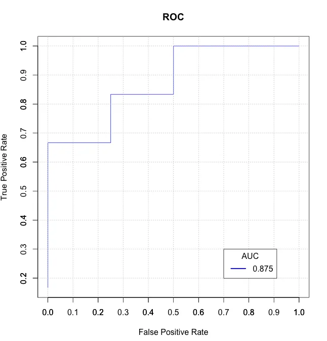
plot(stack_x, stack_y, type = "l", col = "blue", xlab = "False Positive Rate", ylab = "True Positive Rate", main = "ROC")
axis(1, seq(0.0,1.0,0.1))
axis(2, seq(0.0,1.0,0.1))
abline(h=seq(0.0,1.0,0.1), v=seq(0.0,1.0,0.1), col="gray", lty=3)
legend(0.7, 0.3, sprintf("%3.3f",auc), lty=c(1,1), lwd=c(2.5,2.5), col="blue", title = "AUC")

- AGS

---

如果您复制并粘贴此代码，然后收到“Error in plot.window(...) : need finite 'xlim' values”错误提示，那么很可能是因为您的标签是0-1，而@AGS正在使用标签1-2。 - gentimouton

如果两个观察值具有相同的概率且观察顺序不随机，则它不会给出真正的AUC。否则，代码很好且快速。 - MatthieuBizien

不知道为什么这个解决方案在我的数据上不起作用，我的问题没有被归一化到[0,1]范围内。 - Good Will

Answer 5

我发现这里的一些解决方案速度较慢且/或令人困惑（其中一些没有正确处理并列情况），因此我编写了自己基于data.table的函数auc_roc()在我的R包mltools中。

library(data.table)
library(mltools)

preds <- c(.1, .3, .3, .9)
actuals <- c(0, 0, 1, 1)

auc_roc(preds, actuals)  # 0.875

auc_roc(preds, actuals, returnDT=TRUE)
   Pred CountFalse CountTrue CumulativeFPR CumulativeTPR AdditionalArea CumulativeArea
1:  0.9          0         1           0.0           0.5          0.000          0.000
2:  0.3          1         1           0.5           1.0          0.375          0.375
3:  0.1          1         0           1.0           1.0          0.500          0.875

- Ben

---

这个解决方案比pROC包中的auc()方法快得多！如果需要计算多类或多输出回归问题的auc分数，pROC包中的auc()方法相当慢。 - Good Will

Answer 6

您可以通过Miron Kursa的博客文章了解更多关于AUROC的信息：

https://mbq.me/blog/augh-roc/

他提供了一个快速的 AUROC 函数：

# By Miron Kursa https://mbq.me
auroc <- function(score, bool) {
  n1 <- sum(!bool)
  n2 <- sum(bool)
  U  <- sum(rank(score)[!bool]) - n1 * (n1 + 1) / 2
  return(1 - U / n1 / n2)
}

让我们来测试一下：

set.seed(42)
score <- rnorm(1e3)
bool  <- sample(c(TRUE, FALSE), 1e3, replace = TRUE)

pROC::auc(bool, score)
mltools::auc_roc(score, bool)
ROCR::performance(ROCR::prediction(score, bool), "auc")@y.values[[1]]
auroc(score, bool)

0.51371668847094
0.51371668847094
0.51371668847094
0.51371668847094

auroc()比pROC::auc()和computeAUC()快100倍。

auroc()比mltools::auc_roc()和ROCR::performance()快10倍。

print(microbenchmark(
  pROC::auc(bool, score),
  computeAUC(score[bool], score[!bool]),
  mltools::auc_roc(score, bool),
  ROCR::performance(ROCR::prediction(score, bool), "auc")@y.values,
  auroc(score, bool)
))

Unit: microseconds
                                                             expr       min
                                           pROC::auc(bool, score) 21000.146
                            computeAUC(score[bool], score[!bool]) 11878.605
                                    mltools::auc_roc(score, bool)  5750.651
 ROCR::performance(ROCR::prediction(score, bool), "auc")@y.values  2899.573
                                               auroc(score, bool)   236.531
         lq       mean     median        uq        max neval  cld
 22005.3350 23738.3447 22206.5730 22710.853  32628.347   100    d
 12323.0305 16173.0645 12378.5540 12624.981 233701.511   100   c 
  6186.0245  6495.5158  6325.3955  6573.993  14698.244   100  b  
  3019.6310  3300.1961  3068.0240  3237.534  11995.667   100 ab  
   245.4755   253.1109   251.8505   257.578    300.506   100 a   

- Kamil Slowikowski

---

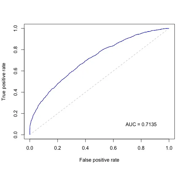
对于更大的样本量，bigstatsr::AUC() 更快（采用C++实现）。免责声明：作者本人。 - F. Privé

Answer 7

结合来自ISL 9.6.3 ROC曲线的代码，以及@J.Won在这个问题中的回答和其他几个地方，以下绘制了ROC曲线，并在图形右下角打印出AUC。

下面probs是二分类预测概率的数字向量，test$label包含测试数据的真实标签。

require(ROCR)
require(pROC)

rocplot <- function(pred, truth, ...) {
  predob = prediction(pred, truth)
  perf = performance(predob, "tpr", "fpr")
  plot(perf, ...)
  area <- auc(truth, pred)
  area <- format(round(area, 4), nsmall = 4)
  text(x=0.8, y=0.1, labels = paste("AUC =", area))

  # the reference x=y line
  segments(x0=0, y0=0, x1=1, y1=1, col="gray", lty=2)
}

rocplot(probs, test$label, col="blue")

这将产生如下图所示的绘图：

- arun

Answer 8

我通常使用DiagnosisMed包中的ROC函数。我喜欢它生成的图形。AUC与其置信区间一起返回，并且也在图形上提到。

ROC(classLabels,scores,Full=TRUE)

- George Dontas

---

截至2016年7月20日，此链接https://cran.r-project.org/web/packages/DiagnosisMed/index.html显示：“‘DiagnosisMed’软件包已从CRAN存储库中删除。” - arun

Answer 9

与Erik的回答类似，您还可以通过比较pos.scores和neg.scores中所有可能的值对来直接计算ROC：

score.pairs <- merge(pos.scores, neg.scores)
names(score.pairs) <- c("pos.score", "neg.score")
sum(score.pairs$pos.score > score.pairs$neg.score) / nrow(score.pairs)

虽然比样本方法或pROC::auc效率低，但比前者更稳定，并且需要的安装工作比后者少。

相关：当我尝试这个方法时，它给出了与pROC值类似的结果，但不完全相同（偏差约为0.02）；结果更接近于具有非常高N的样本方法。如果有人有想法为什么会这样，我会感兴趣。

- Max Ghenis

---

不准确性的一个来源是处理并列情况。严格来说，应该计算正例得分严格大于反例得分的概率加上相等的概率的一半。如果所有得分都是唯一的，则不会有问题。 - user2920554

Answer 10

目前得票最高的答案是不正确的，因为它忽略了并列情况。当正分数和负分数相等时，AUC应该为0.5。下面是更正后的示例。

computeAUC <- function(pos.scores, neg.scores, n_sample=100000) {
  # Args:
  #   pos.scores: scores of positive observations
  #   neg.scores: scores of negative observations
  #   n_samples : number of samples to approximate AUC

  pos.sample <- sample(pos.scores, n_sample, replace=T)
  neg.sample <- sample(neg.scores, n_sample, replace=T)
  mean(1.0*(pos.sample > neg.sample) + 0.5*(pos.sample==neg.sample))
}

- Jussi Kujala