分段仿射变换+扭曲输出看起来很奇怪。

Question

分段仿射变换+扭曲输出看起来很奇怪。

pythonpython-2.7numpyaffinetransformscikit-image

5

我正在尝试使用skimage.PiecewiseAffineTransform和skimage.warp来扭曲一张图片。我有一组控制点（true）映射到一个新的控制点集合（ideal），但扭曲并没有返回我期望的结果。

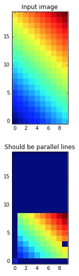
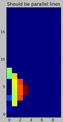
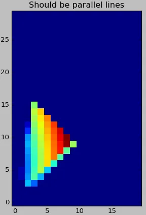
在这个例子中，我有一个简单的波长梯度，我试图将其“拉直”成列。（你可能会问为什么我要找轮廓和插值，但那是因为我实际上将这个代码应用于更复杂的用例。我只是想为这个简单的例子复制所有代码，以产生相同奇怪的输出。）

任何原因导致我的输出图像只有输入图像被扭曲成正方形和嵌入内部？我正在使用Python 2.7.12和matplotlib 1.5.1。以下是代码。

import matplotlib.pyplot as plt
import numpy as np
from skimage import measure, transform

true = np.array([range(i,i+10) for i in range(20)])
ideal = np.array([range(10)]*20)

# Find contours of ideal and true images and create list of control points for warp
true_control_pts = []
ideal_control_pts = []

for lam in ideal[0]:
    try:
        # Get the isowavelength contour in the true and ideal images
        tc = measure.find_contours(true, lam)[0]
        ic = measure.find_contours(ideal, lam)[0]
        nc = np.ones(ic.shape)

        # Use the y coordinates of the ideal contour
        nc[:, 0] = ic[:, 0]

        # Interpolate true contour onto ideal contour y axis so there are the same number of points
        nc[:, 1] = np.interp(ic[:, 0], tc[:, 0], tc[:, 1])

        # Add the control points to the appropriate list
        true_control_pts.append(nc.tolist())
        ideal_control_pts.append(ic.tolist())

    except (IndexError,AttributeError):
        pass

true_control_pts = np.array(true_control_pts)
ideal_control_pts = np.array(ideal_control_pts)

length = len(true_control_pts.flatten())/2
true_control_pts = true_control_pts.reshape(length,2)
ideal_control_pts = ideal_control_pts.reshape(length,2)

# Plot the original image
image = np.array([range(i,i+10) for i in range(20)]).astype(np.int32)
plt.figure()
plt.imshow(image, origin='lower', interpolation='none')
plt.title('Input image')

# Warp the actual image given the transformation between the true and ideal wavelength maps
tform = transform.PiecewiseAffineTransform()
tform.estimate(true_control_pts, ideal_control_pts)
out = transform.warp(image, tform)

# Plot the warped image!
fig, ax = plt.subplots()
ax.imshow(out, origin='lower', interpolation='none')
plt.title('Should be parallel lines')

这个的输出结果如下所示:

非常感谢您的帮助！

- Joe Flip

尚未测试，但有一件事引起了注意 - 输出图使用了subplot。首先要尝试的是使用plt.figure / plt.imshow绘制变形图像，而不是使用plt.subplots / ax.imshow。另外，请编辑您的问题以包含您的“import”语句？谢谢！还有，使用的Python版本是什么？ - cxw

@cxw 更新了，谢谢！ - Joe Flip

@cxw 尝试过不使用 plt.subplots()，但结果相同。 - Joe Flip

回答已发布！我明天到周日都会离开电脑。希望以下内容能帮助您找出实际使用情况中发生的问题！ - cxw

1个回答

网页内容由stack overflow 提供, 点击上面的

可以查看英文原文，
原文链接

- cxw · Accepted Answer

我会提供给你我所拥有的内容。考虑到所给的测试数据，我不认为我能够准确地完成此项任务。在这样一个小图像中将45度角映射到直线意味着需要进行大量运动，但可用数据很少。我在下面的代码中发现了一些特定的错误，并进行了修复，标记为/* */（因为这不是Python文件中通常看到的东西，所以该标记应该很突出 :)）。

请在真实数据上尝试这段代码，并告诉我它是否有效！对于这个输入数据集，存在一些非零输出。

主要问题如下：

interp数据需要排序
许多控制点是荒谬的，因为这个数据集中的数据不足（例如，将一列的大跨度映射到单个点）
图像中的值范围偏离了（因此您原来的输出实际上几乎全部为0-颜色补丁的值约为1e-9）。

我添加的最重要的内容是一个3D图，显示“真实”控制点如何映射到“理想”控制点，这为您提供了一个调试工具，以便您了解控制点映射是否符合预期。这个图表是导致我遇到interp问题的原因。

顺便说一下，请使用“before”和“after”等名称，而不是ideal和true :)。至少有一次，我试图记住哪个是哪个，结果被绊倒了。

第一次尝试

import pdb
import matplotlib.pyplot as plt
import numpy as np
from skimage import measure, transform, img_as_float

from mpl_toolkits.mplot3d import Axes3D # /**/

#/**/
# From https://dev59.com/THI95IYBdhLWcg3wyBCc#14491059 by
# https://stackoverflow.com/users/1355221/dansalmo
def flatten_list(L):
    for item in L:
        try:
            for i in flatten_list(item): yield i
        except TypeError:
            yield item
#end flatten_list

true_input = np.array([range(i,i+10) for i in range(20)])  # /** != True **/
ideal = np.array([range(10)]*20)

#pdb.set_trace()
# Find contours of ideal and true_input images and create list of control points for warp
true_control_pts = []
ideal_control_pts = []
OLD_true=[]     # /**/ for debugging
OLD_ideal=[]

for lam in [x+0.5 for x in ideal[0]]:   # I tried the 0.5 offset just to see,
    try:                                # but it didn't make much difference

        # Get the isowavelength contour in the true_input and ideal images
        tc = measure.find_contours(true_input, lam)[0]
        ic = measure.find_contours(ideal, lam)[0]
        nc = np.zeros(ic.shape) # /** don't need ones() **/

        # Use the y /** X? **/ coordinates of the ideal contour
        nc[:, 0] = ic[:, 0]

        # Interpolate true contour onto ideal contour y axis so there are the same number of points

        # /** Have to sort first - https://docs.scipy.org/doc/numpy/reference/generated/numpy.interp.html#numpy-interp **/
        tc_sorted = tc[tc[:,0].argsort()]
            # /** Thanks to https://dev59.com/SXE85IYBdhLWcg3wVR-g#2828121 by
            # https://stackoverflow.com/users/208339/steve-tjoa **/

        nc[:, 1] = np.interp(ic[:, 0], tc_sorted[:, 0], tc_sorted[:, 1],
            left=np.nan, right=np.nan)
            # /** nan: If the interpolation is out of range, we're not getting
            #     useful data.  Therefore, flag it with a nan. **/

        # /** Filter out the NaNs **/
        # Thanks to https://dev59.com/O2gu5IYBdhLWcg3wRlBh#11453235 by
        # https://stackoverflow.com/users/449449/eumiro
        #pdb.set_trace()
        indices = ~np.isnan(nc).any(axis=1)
        nc_nonan = nc[indices]
        ic_nonan = ic[indices]

        # Add the control points to the appropriate list.
        # /** Flattening here since otherwise I wound up with dtype=object
        #     in the numpy arrays. **/
        true_control_pts.append(nc_nonan.flatten().tolist())
        ideal_control_pts.append(ic_nonan.flatten().tolist())

        OLD_true.append(nc)     # /** for debug **/
        OLD_ideal.append(ic)

    except (IndexError,AttributeError):
        pass

#pdb.set_trace()
# /** Make vectors of all the control points. **/
true_flat = list(flatten_list(true_control_pts))
ideal_flat = list(flatten_list(ideal_control_pts))
true_control_pts = np.array(true_flat)
ideal_control_pts = np.array(ideal_flat)

# Make the vectors 2d
length = len(true_control_pts)/2
true_control_pts = true_control_pts.reshape(length,2)
ideal_control_pts = ideal_control_pts.reshape(length,2)

#pdb.set_trace()

# Plot the original image
image = np.array([range(i,i+10) for i in range(20)]) / 30.0 # /**.astype(np.int32)**/
    # /** You don't want int32 images!  See
    #     http://scikit-image.org/docs/dev/user_guide/data_types.html .
    #     Manually rescale the image to [0.0,1.0] by dividing by 30. **/
image_float = img_as_float(image) #/** make sure skimage is happy */ 
fig = plt.figure()
plt.imshow(image_float, origin='lower', interpolation='none')
plt.title('Input image')
fig.show()  # /** I needed this on my test system **/

# Warp the actual image given the transformation between the true and ideal wavelength maps
tform = transform.PiecewiseAffineTransform()
tform.estimate(true_control_pts, ideal_control_pts)
out = transform.warp(image, tform)
    # /** since we started with float, and this is float, too, the two are
    #     comparable. **/

pdb.set_trace()

# Plot the warped image!
fig, ax = plt.subplots()
ax.imshow(out, origin='lower', interpolation='none')    # /**note: float**/
plt.title('Should be parallel lines')
fig.show()

# /** Show the control points.
#     The z=0 plane will be the "true" control points (before), and the
#     z=1 plane will be the "ideal" control points (after). **/
fig = plt.figure()
ax = fig.add_subplot(111, projection='3d')
fig.show()

for rowidx in range(length):
    ax.plot([true_control_pts[rowidx,0], ideal_control_pts[rowidx,0]],
            [true_control_pts[rowidx,1], ideal_control_pts[rowidx,1]],
            [0,1])

input() # /** because I was running from the command line **/

第二次尝试

越来越接近：

这里是控制点映射的视图，看起来更加有前途：

你可以看到它试图旋转图像一点，这正是我从这个数据集所期望的。

代码

import pdb
import matplotlib.pyplot as plt
import numpy as np
from skimage import measure, transform, img_as_float

from mpl_toolkits.mplot3d import Axes3D # /**/

#/**/
# From https://dev59.com/THI95IYBdhLWcg3wyBCc#14491059 by
# https://stackoverflow.com/users/1355221/dansalmo
def flatten_list(L):
    for item in L:
        try:
            for i in flatten_list(item): yield i
        except TypeError:
            yield item
#end flatten_list

#/**/
# Modified from https://dev59.com/0mIk5IYBdhLWcg3wn_RF#19122075 by
# https://stackoverflow.com/users/2588210/christian-k
def equispace(data, npts):
    x,y = data.T
    xd =np.diff(x)
    yd = np.diff(y)
    dist = np.sqrt(xd**2+yd**2)
    u = np.cumsum(dist)
    u = np.hstack([[0],u])

    t = np.linspace(0,u.max(),npts)
    xn = np.interp(t, u, x)
    yn = np.interp(t, u, y)
    return np.column_stack((xn, yn))

true_input = np.array([range(i,i+10) for i in range(20)])  # /** != True **/
ideal = np.array([range(10)]*20)

#pdb.set_trace()
# Find contours of ideal and true_input images and create list of control points for warp
true_control_pts = []
ideal_control_pts = []
OLD_true=[]     # /**/ for debugging
OLD_ideal=[]

for lam in [x+0.5 for x in ideal[0]]:   # I tried the 0.5 offset just to see,
    try:                                # but it didn't make much difference

        # Get the isowavelength contour in the true_input and ideal images
        tc = measure.find_contours(true_input, lam)[0]
            # /** So this might not have very many numbers in it. **/
        ic = measure.find_contours(ideal, lam)[0]
            # /** CAUTION: this is assuming the contours are going the same
            #       direction.  If not, you'll need to make it so. **/
        #nc = np.zeros(ic.shape) # /** don't need ones() **/

        # /** We just want to find points on _tc_ to match _ic_.  That's
        #       interpolation _within_ a curve. **/
        #pdb.set_trace()
        nc_by_t = equispace(tc,ic.shape[0])
        ic_by_t = equispace(ic,ic.shape[0])


        ### /** Not this **/
        ## Use the y /** X? **/ coordinates of the ideal contour
        #nc[:, 0] = ic[:, 0]
        #
        ## Interpolate true contour onto ideal contour y axis so there are the same number of points
        #
        ## /** Have to sort first - https://docs.scipy.org/doc/numpy/reference/generated/numpy.interp.html#numpy-interp **/
        #tc_sorted = tc[tc[:,0].argsort()]
        #    # /** Thanks to https://dev59.com/SXE85IYBdhLWcg3wVR-g#2828121 by
        #    # https://stackoverflow.com/users/208339/steve-tjoa **/
        #
        #nc[:, 1] = np.interp(ic[:, 0], tc_sorted[:, 0], tc_sorted[:, 1],
        #    left=np.nan, right=np.nan)
        #    # /** nan: If the interpolation is out of range, we're not getting
        #    #     useful data.  Therefore, flag it with a nan. **/

        # /** Filter out the NaNs **/
        # Thanks to https://dev59.com/O2gu5IYBdhLWcg3wRlBh#11453235 by
        # https://stackoverflow.com/users/449449/eumiro
        #pdb.set_trace()
        #indices = ~np.isnan(nc).any(axis=1)
        #nc_nonan = nc[indices]
        #ic_nonan = ic[indices]
        #

        # Add the control points to the appropriate list.
        ## /** Flattening here since otherwise I wound up with dtype=object
        ##     in the numpy arrays. **/
        #true_control_pts.append(nc_nonan.flatten().tolist())
        #ideal_control_pts.append(ic_nonan.flatten().tolist())

        #OLD_true.append(nc)     # /** for debug **/
        #OLD_ideal.append(ic)

        true_control_pts.append(nc_by_t)
        ideal_control_pts.append(ic_by_t)

    except (IndexError,AttributeError):
        pass

pdb.set_trace()
# /** Make vectors of all the control points. **/
true_flat = list(flatten_list(true_control_pts))
ideal_flat = list(flatten_list(ideal_control_pts))
true_control_pts = np.array(true_flat)
ideal_control_pts = np.array(ideal_flat)

# Make the vectors 2d
length = len(true_control_pts)/2
true_control_pts = true_control_pts.reshape(length,2)
ideal_control_pts = ideal_control_pts.reshape(length,2)

#pdb.set_trace()

# Plot the original image
image = np.array([range(i,i+10) for i in range(20)]) / 30.0 # /**.astype(np.int32)**/
    # /** You don't want int32 images!  See
    #     http://scikit-image.org/docs/dev/user_guide/data_types.html .
    #     Manually rescale the image to [0.0,1.0] by dividing by 30. **/
image_float = img_as_float(image) #/** make sure skimage is happy */ 
fig = plt.figure()
plt.imshow(image_float, origin='lower', interpolation='none')
plt.title('Input image')
fig.show()  # /** I needed this on my test system **/

# Warp the actual image given the transformation between the true and ideal wavelength maps
tform = transform.PiecewiseAffineTransform()
tform.estimate(true_control_pts, ideal_control_pts)
out = transform.warp(image, tform)
    # /** since we started with float, and this is float, too, the two are
    #     comparable. **/

pdb.set_trace()

# Plot the warped image!
fig, ax = plt.subplots()
ax.imshow(out, origin='lower', interpolation='none')    # /**note: float**/
plt.title('Should be parallel lines')
fig.show()

# /** Show the control points.
#     The z=0 plane will be the "true" control points (before), and the
#     z=1 plane will be the "ideal" control points (after). **/
fig = plt.figure()
ax = fig.add_subplot(111, projection='3d')
fig.show()

for rowidx in range(length):
    ax.plot([true_control_pts[rowidx,0], ideal_control_pts[rowidx,0]],
            [true_control_pts[rowidx,1], ideal_control_pts[rowidx,1]],
            [0,1])

input() # /** because I was running from the command line **/

解释

从不同的角度考虑插值：您实际上想要映射的并不是 X 和 Y 坐标，对吗？我认为您想要映射的是沿轮廓的距离，以便将对角线轮廓拉伸为垂直轮廓。这就是这些行所做的事情：

nc_by_t = equispace(tc,ic.shape[0])
ic_by_t = equispace(ic,ic.shape[0])

我们沿着每个轮廓线制作ic.shape[0]数量的等间距点，然后将这些点映射到彼此。 equispace是从this answer修改而来。因此，这将缩短轮廓线以适应更长的轮廓线，无论哪种方式，点数由ic中定义的轮廓线长度确定。实际上，您可以使用任意数量的点进行此技术；我只测试了100个点，并获得了基本相同的结果。

再次，在您的实际数据上测试此方法。仔细考虑插值的参考是什么。它真的是X或Y坐标吗？是沿轮廓线的距离吗？是轮廓线的百分比（如上所述）吗？

好的，再提供一个想法

对于这个特定的测试案例，是否需要更多数据？是的！

我使用较大的图像确定控制点，然后将一个较小的图像映射到该区域的中心。

代码

（到此为止，代码已经一团糟 - 请参见===========标记）

import pdb
import matplotlib.pyplot as plt
import numpy as np
from skimage import measure, transform, img_as_float

from mpl_toolkits.mplot3d import Axes3D # /**/

#/**/
def test_figure(data,title):
    image_float = img_as_float(data) #/** make sure skimage is happy */ 
    fig = plt.figure()
    plt.imshow(image_float, origin='lower', interpolation='none')
    plt.title(title)
    fig.show()

#/**/
# From https://dev59.com/THI95IYBdhLWcg3wyBCc#14491059 by
# https://stackoverflow.com/users/1355221/dansalmo
def flatten_list(L):
    for item in L:
        try:
            for i in flatten_list(item): yield i
        except TypeError:
            yield item
#end flatten_list

#/**/
# Modified from https://dev59.com/0mIk5IYBdhLWcg3wn_RF#19122075 by
# https://stackoverflow.com/users/2588210/christian-k
def equispace(data, npts):
    x,y = data.T
    xd =np.diff(x)
    yd = np.diff(y)
    dist = np.sqrt(xd**2+yd**2)
    u = np.cumsum(dist)
    u = np.hstack([[0],u])

    t = np.linspace(0,u.max(),npts)
    xn = np.interp(t, u, x)
    yn = np.interp(t, u, y)
    return np.column_stack((xn, yn))

# ======================  BIGGER
true_input = np.array([range(i,i+20) for i in range(30)])  # /** != True **/
ideal = np.array([range(20)]*30)
# ======================    
test_figure(true_input / 50.0, 'true_input')
test_figure(ideal / 20.0, 'ideal')

#pdb.set_trace()
# Find contours of ideal and true_input images and create list of control points for warp
true_control_pts = []
ideal_control_pts = []
OLD_true=[]     # /**/ for debugging
OLD_ideal=[]

for lam in [x+0.5 for x in ideal[0]]:   # I tried the 0.5 offset just to see,
    try:                                # but it didn't make much difference

        # Get the isowavelength contour in the true_input and ideal images
        tc = measure.find_contours(true_input, lam)[0]
            # /** So this might not have very many numbers in it. **/
        ic = measure.find_contours(ideal, lam)[0]
            # /** CAUTION: this is assuming the contours are going the same
            #       direction.  If not, you'll need to make it so. **/
        #nc = np.zeros(ic.shape) # /** don't need ones() **/

        # /** We just want to find points on _tc_ to match _ic_.  That's
        #       interpolation _within_ a curve. **/
        #pdb.set_trace()
        nc_by_t = equispace(tc,ic.shape[0])
        ic_by_t = equispace(ic,ic.shape[0])


        ### /** Not this **/
        ## Use the y /** X? **/ coordinates of the ideal contour
        #nc[:, 0] = ic[:, 0]
        #
        ## Interpolate true contour onto ideal contour y axis so there are the same number of points
        #
        ## /** Have to sort first - https://docs.scipy.org/doc/numpy/reference/generated/numpy.interp.html#numpy-interp **/
        #tc_sorted = tc[tc[:,0].argsort()]
        #    # /** Thanks to https://dev59.com/SXE85IYBdhLWcg3wVR-g#2828121 by
        #    # https://stackoverflow.com/users/208339/steve-tjoa **/
        #
        #nc[:, 1] = np.interp(ic[:, 0], tc_sorted[:, 0], tc_sorted[:, 1],
        #    left=np.nan, right=np.nan)
        #    # /** nan: If the interpolation is out of range, we're not getting
        #    #     useful data.  Therefore, flag it with a nan. **/

        # /** Filter out the NaNs **/
        # Thanks to https://dev59.com/O2gu5IYBdhLWcg3wRlBh#11453235 by
        # https://stackoverflow.com/users/449449/eumiro
        #pdb.set_trace()
        #indices = ~np.isnan(nc).any(axis=1)
        #nc_nonan = nc[indices]
        #ic_nonan = ic[indices]
        #

        # Add the control points to the appropriate list.
        ## /** Flattening here since otherwise I wound up with dtype=object
        ##     in the numpy arrays. **/
        #true_control_pts.append(nc_nonan.flatten().tolist())
        #ideal_control_pts.append(ic_nonan.flatten().tolist())

        #OLD_true.append(nc)     # /** for debug **/
        #OLD_ideal.append(ic)

        true_control_pts.append(nc_by_t)
        ideal_control_pts.append(ic_by_t)

    except (IndexError,AttributeError):
        pass

#pdb.set_trace()
# /** Make vectors of all the control points. **/
true_flat = list(flatten_list(true_control_pts))
ideal_flat = list(flatten_list(ideal_control_pts))
true_control_pts = np.array(true_flat)
ideal_control_pts = np.array(ideal_flat)

# Make the vectors 2d
length = len(true_control_pts)/2
true_control_pts = true_control_pts.reshape(length,2)
ideal_control_pts = ideal_control_pts.reshape(length,2)

#pdb.set_trace()

# Plot the original image
image = np.array([range(i,i+10) for i in range(20)]) / 30.0 # /**.astype(np.int32)**/
    # /** You don't want int32 images!  See
    #     http://scikit-image.org/docs/dev/user_guide/data_types.html .
    #     Manually rescale the image to [0.0,1.0] by dividing by 30. **/

# ======================    
# /** Pad from 10x20 to 20x30 just for grins **/
#pdb.set_trace()
image = np.concatenate( (np.zeros((20,5)),image,np.zeros((20,5))), 1)
    # now it's 20x20
image = np.concatenate( (np.zeros((5,20)),image,np.zeros((5,20))), 0)
# ======================    

#Plot it
image_float = img_as_float(image) #/** make sure skimage is happy */ 
fig = plt.figure()
plt.imshow(image_float, origin='lower', interpolation='none')
plt.title('Input image')
fig.show()  # /** I needed this on my test system **/

# Warp the actual image given the transformation between the true and ideal wavelength maps
tform = transform.PiecewiseAffineTransform()
tform.estimate(true_control_pts, ideal_control_pts)
out = transform.warp(image, tform)
    # /** since we started with float, and this is float, too, the two are
    #     comparable. **/

pdb.set_trace()

# Plot the warped image!
fig, ax = plt.subplots()
ax.imshow(out, origin='lower', interpolation='none')    # /**note: float**/
plt.title('Should be parallel lines')
fig.show()

# /** Show the control points.
#     The z=0 plane will be the "true" control points (before), and the
#     z=1 plane will be the "ideal" control points (after). **/
fig = plt.figure()
ax = fig.add_subplot(111, projection='3d')
fig.show()

for rowidx in range(length):
    ax.plot([true_control_pts[rowidx,0], ideal_control_pts[rowidx,0]],
            [true_control_pts[rowidx,1], ideal_control_pts[rowidx,1]],
            [0,1])

input() # /** because I was running from the command line **/