OpenCV在图像上检测斑点

Question

我需要找到图像中的最大和最小半径的blob，并在它们周围画一个矩形。(下面有示例)

问题是要为图像找到正确的过滤器，使得Canny或Threshold变换可以突出显示这些blob。然后我将使用findContours找到矩形。

我已经尝试过:

• Threshold - 使用不同的级别

• 模糊->腐蚀->腐蚀->灰度->Canny

• 使用各种“线条”改变图像色调

等等。更好的结果是检测到了blob的一部分（20-30％）。而这些信息不能够绘制一个完整的矩形。此外，由于阴影的影响，与blob无关的点也被检测到了，这也防止了检测区域。

据我所知，我需要找到具有硬对比度（不像阴影中那样平滑）的轮廓。有没有用openCV实现这个功能的方法？

更新

分别处理这些案例：图1、图2、图3、图4、图5、图6、图7、图8、图9、图10、图11、图12

另外补充一下

我认为斑块在边缘处具有对比度区域。因此，我尝试加强边缘：我创建了两个灰度Mat：A和B，对第二个应用高斯模糊 - B（稍微减少一些噪声），然后进行了一些计算：绕着每个像素走，并查找'A'和'B'中附近点之间的Xi,Yi的最大差异：

并将Xi,Yi之间的max差异应用。我得到了以下结果：

是否正确？顺便问一下，我能通过OpenCV方法实现这样的效果吗？

更新:图像去噪有助于降低噪音，Sobel突出轮廓，然后使用threshold+findContours和custome convexHull可以得到类似于我要找的结果，但对于某些斑点效果不好。

- Siarhei

---

为什么输入是以拼贴的形式呈现的？这是原始输入格式吗？还是您自己创建了一种格式来展示不同的情况？ - ZdaR

@ZdaR 是的，我创建它是为了展示不同的情况。并不是所有可能的变体都包含在内（但我希望包含了最流行的）。 - Siarhei

你能把所有的案例分别上传吗？ - ZdaR

@ZdaR，已将输入文件分别上传到 i.stack.imgur.com，谢谢。 - Siarhei

恭喜，你刚刚（重新）发现了高通滤波器！当你从原始图像中减去高斯模糊时，边缘会产生高响应...具体而言，使其困难的是反射也有锐利的边缘。 - Eran W

Answer 1

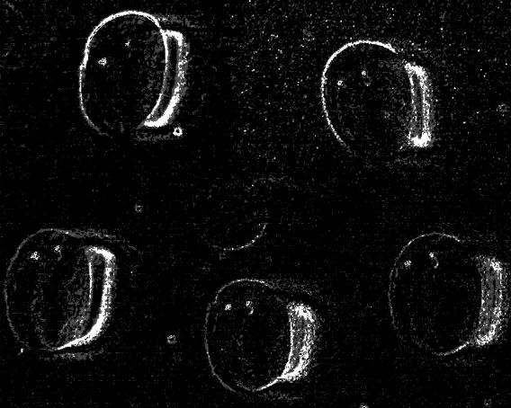
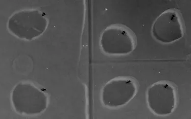
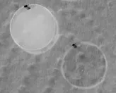
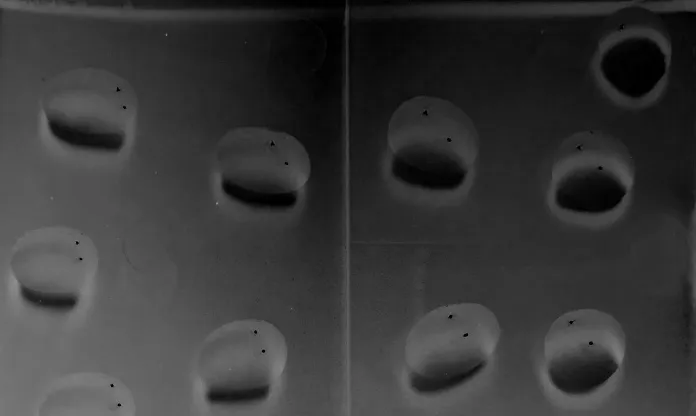
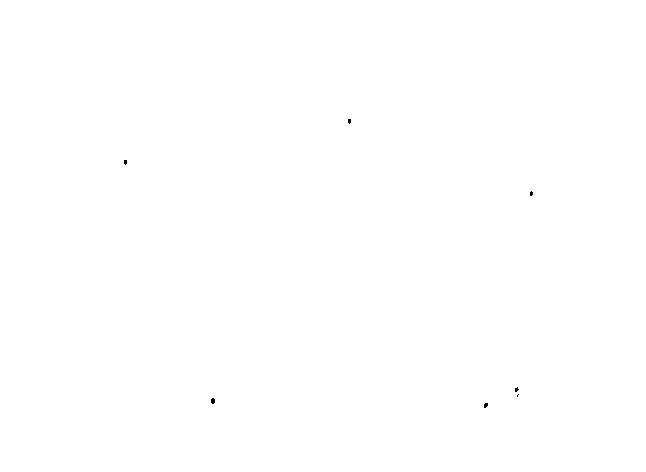
由于输入图像之间存在很大的差异，算法应该能够适应各种情况。由于Canny算法基于检测高频率，我的算法将图像的锐度作为预处理适应的参数。我不想花费一周时间来找出所有数据的函数，所以我应用了一个简单的线性函数，基于两个图像，然后用第三个图像进行测试。以下是我的结果:

请注意，这只是一种基本方法，仅用于证明一个观点。它需要实验、测试和改进。该想法是使用Sobel算子，并对获取的所有像素求和。将其除以图像的大小，应该可以基本估计图像的高频响应。现在，通过实验，我找到了适用于CLAHE滤波器的clipLimit值，在两个测试案例中发现了与输入的高频响应连接的线性函数，产生了良好的结果。

sobel = get_sobel(img)
clip_limit = (-2.556) * np.sum(sobel)/(img.shape[0] * img.shape[1]) + 26.557

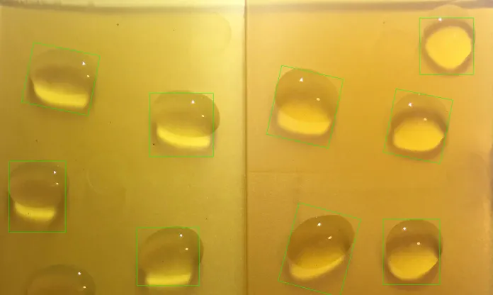
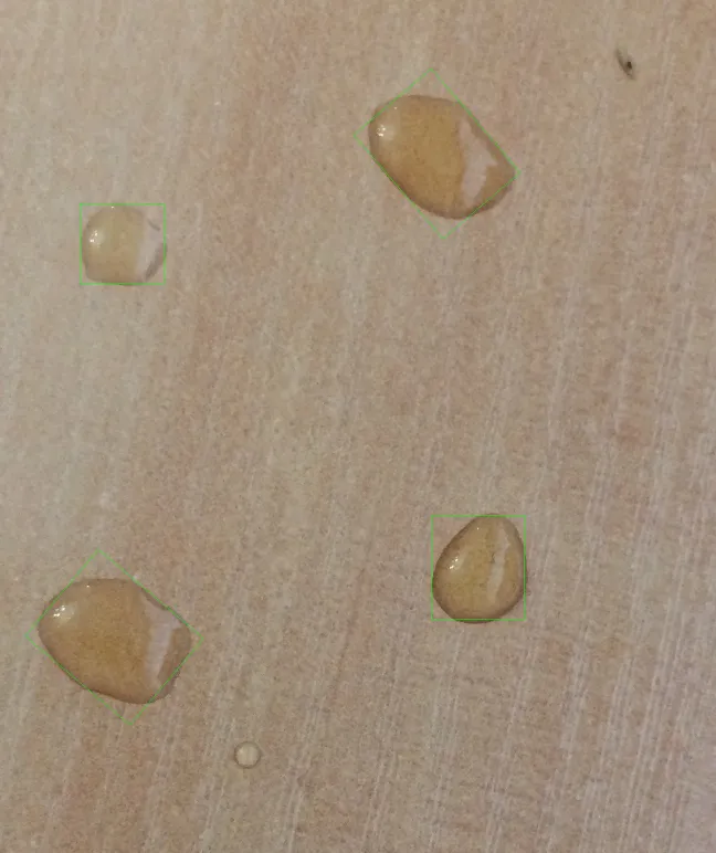
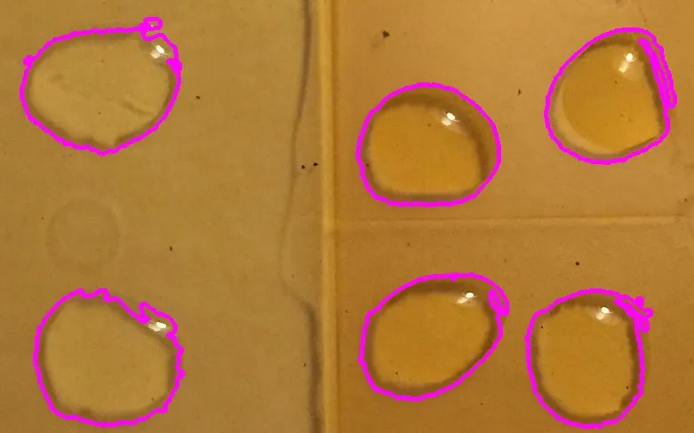
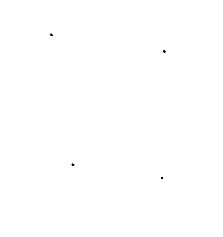
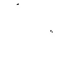
那是自适应部分。现在来说轮廓。我花了一些时间才找到一种正确的方法来过滤噪音。我选择了一个简单的技巧：使用两次轮廓查找。首先，我使用它来滤掉不必要的嘈杂轮廓。然后，我继续使用一些形态学魔术，以得到正确的对象检测斑点（代码中有更多详细信息）。最后一步是根据计算出的平均值过滤边界矩形，因为在所有样本中，斑点的大小相对较为相似。

import cv2
import numpy as np


def unsharp_mask(img, blur_size = (5,5), imgWeight = 1.5, gaussianWeight = -0.5):
    gaussian = cv2.GaussianBlur(img, (5,5), 0)
    return cv2.addWeighted(img, imgWeight, gaussian, gaussianWeight, 0)


def smoother_edges(img, first_blur_size, second_blur_size = (5,5), imgWeight = 1.5, gaussianWeight = -0.5):
    img = cv2.GaussianBlur(img, first_blur_size, 0)
    return unsharp_mask(img, second_blur_size, imgWeight, gaussianWeight)


def close_image(img, size = (5,5)):
    kernel = np.ones(size, np.uint8)
    return cv2.morphologyEx(img, cv2.MORPH_CLOSE, kernel)


def open_image(img, size = (5,5)):
    kernel = np.ones(size, np.uint8)
    return cv2.morphologyEx(img, cv2.MORPH_OPEN, kernel)


def shrink_rect(rect, scale = 0.8):
    center, (width, height), angle = rect
    width = width * scale
    height = height * scale
    rect = center, (width, height), angle
    return rect


def clahe(img, clip_limit = 2.0):
    clahe = cv2.createCLAHE(clipLimit=clip_limit, tileGridSize=(5,5))
    return clahe.apply(img)


def get_sobel(img, size = -1):
    sobelx64f = cv2.Sobel(img,cv2.CV_64F,2,0,size)
    abs_sobel64f = np.absolute(sobelx64f)
    return np.uint8(abs_sobel64f)


img = cv2.imread("blobs4.jpg")
# save color copy for visualizing
imgc = img.copy()
# resize image to make the analytics easier (a form of filtering)
resize_times = 5
img = cv2.resize(img, None, img, fx = 1 / resize_times, fy = 1 / resize_times)
img = cv2.cvtColor(img, cv2.COLOR_BGR2GRAY)

# use sobel operator to evaluate high frequencies
sobel = get_sobel(img)
# experimentally calculated function - needs refining
clip_limit = (-2.556) * np.sum(sobel)/(img.shape[0] * img.shape[1]) + 26.557

# don't apply clahe if there is enough high freq to find blobs
if(clip_limit < 1.0):
    clip_limit = 0.1
# limit clahe if there's not enough details - needs more tests
if(clip_limit > 8.0):
    clip_limit = 8

# apply clahe and unsharp mask to improve high frequencies as much as possible
img = clahe(img, clip_limit)
img = unsharp_mask(img)

# filter the image to ensure edge continuity and perform Canny
# (values selected experimentally, using trackbars)
img_blurred = (cv2.GaussianBlur(img.copy(), (2*2+1,2*2+1), 0))
canny = cv2.Canny(img_blurred, 35, 95)

# find first contours
_, cnts, _ = cv2.findContours(canny.copy(), cv2.RETR_LIST, cv2.CHAIN_APPROX_SIMPLE)

# prepare black image to draw contours
canvas = np.ones(img.shape, np.uint8)
for c in cnts:
    l = cv2.arcLength(c, False)
    x,y,w,h = cv2.boundingRect(c)
    aspect_ratio = float(w)/h

    # filter "bad" contours (values selected experimentally)
    if l > 500:
        continue
    if l < 20:
        continue
    if aspect_ratio < 0.2:
        continue
    if aspect_ratio > 5:
        continue
    if l > 150 and (aspect_ratio > 10 or aspect_ratio < 0.1):
        continue
    # draw all the other contours
    cv2.drawContours(canvas, [c], -1, (255, 255, 255), 2)

# perform closing and blurring, to close the gaps
canvas = close_image(canvas, (7,7))
img_blurred = cv2.GaussianBlur(canvas, (8*2+1,8*2+1), 0)
# smooth the edges a bit to make sure canny will find continuous edges
img_blurred = smoother_edges(img_blurred, (9,9))
kernel = np.ones((3,3), np.uint8)
# erode to make sure separate blobs are not touching each other
eroded = cv2.erode(img_blurred, kernel)
# perform necessary thresholding before Canny
_, im_th = cv2.threshold(eroded, 50, 255, cv2.THRESH_BINARY)
canny = cv2.Canny(im_th, 11, 33)

# find contours again. this time mostly the right ones
_, cnts, _ = cv2.findContours(canny.copy(), cv2.RETR_EXTERNAL, cv2.CHAIN_APPROX_SIMPLE)

# calculate the mean area of the contours' bounding rectangles
sum_area = 0
rect_list = []
for i,c in enumerate(cnts):
    rect = cv2.minAreaRect(c)
    _, (width, height), _ = rect
    area = width*height
    sum_area += area
    rect_list.append(rect)
mean_area = sum_area / len(cnts)

# choose only rectangles that fulfill requirement:
# area > mean_area*0.6
for rect in rect_list:
    _, (width, height), _ = rect
    box = cv2.boxPoints(rect)
    box = np.int0(box * 5)
    area = width * height

    if(area > mean_area*0.6):
        # shrink the rectangles, since the shadows and reflections
        # make the resulting rectangle a bit bigger
        # the value was guessed - might need refinig
        rect = shrink_rect(rect, 0.8)
        box = cv2.boxPoints(rect)
        box = np.int0(box * resize_times)
        cv2.drawContours(imgc, [box], 0, (0,255,0),1)

# resize for visualizing purposes
imgc = cv2.resize(imgc, None, imgc, fx = 0.5, fy = 0.5)
cv2.imshow("imgc", imgc)
cv2.imwrite("result3.png", imgc)
cv2.waitKey(0)

总的来说，我认为这是一个非常有趣的问题，但涉及面有点太广，无法在此回答。我提出的方法只能作为路标而不是完整的解决方案。其基本思想是：

1. 自适应预处理。

2. 两次查找轮廓：一次用于过滤，一次用于实际分类。

3. 根据均值大小过滤斑点。

感谢您的阅读，祝好运！

- m3h0w

---

谢谢!很棒的答案。可以再加上一次赏金吗? - Siarhei

@user5599807 我不知道 :) 不客气 - 这很有趣。 - Michał Gacka

Answer 2

这是我使用的代码：

import cv2
from sympy import Point, Ellipse
import numpy as np
x1='C:\\Users\\Desktop\\python\\stack_over_flow\\XsXs9.png'    
image = cv2.imread(x1,0)
image1 = cv2.imread(x1,1)
x,y=image.shape
median = cv2.GaussianBlur(image,(9,9),0)
median1 = cv2.GaussianBlur(image,(21,21),0)
a=median1-median
c=255-a
ret,thresh1 = cv2.threshold(c,12,255,cv2.THRESH_BINARY)
kernel=np.ones((5,5),np.uint8)
dilation = cv2.dilate(thresh1,kernel,iterations = 1)
kernel=np.ones((5,5),np.uint8)
opening = cv2.morphologyEx(dilation, cv2.MORPH_OPEN, kernel)
cv2.imwrite('D:\\test12345.jpg',opening)
ret,contours,hierarchy =    cv2.findContours(opening,cv2.RETR_EXTERNAL,cv2.CHAIN_APPROX_SIMPLE)
c=np.size(contours[:])
Blank_window=np.zeros([x,y,3])
Blank_window=np.uint8(Blank_window)
for u in range(0,c-1):
    if (np.size(contours[u])>200):
        ellipse = cv2.fitEllipse(contours[u])
        (center,axes,orientation) =ellipse
        majoraxis_length = max(axes)
        minoraxis_length = min(axes)
        eccentricity=(np.sqrt(1-(minoraxis_length/majoraxis_length)**2))
        if (eccentricity<0.8):
             cv2.drawContours(image1, contours, u, (255,1,255), 3)
cv2.imwrite('D:\\marked.jpg',image1)

问题是寻找一个近似圆形的对象。这个简单的解决方案是基于找到每个轮廓的离心率。如图所示，被检测到的对象是一滴水。

- K.Sarkar

---

不错的方法，使用离心率。 - Jeru Luke

我认为这并没有实际解决问题。这个答案的作者只使用了几个最简单的情况。这里的问题主要在于反射、不同的背景和整体噪音。在我看来，这些操作至少会在问题中展示的30%的情况下失败。使用了其中一个案例的代码。 - Michał Gacka

是的，这并不适用于所有图像，但看起来是真实的 - 应该有几个算法和逻辑来检测应该应用于某些类型的图像。此外，这种解决方案在某些情况下具有高精度。看起来我需要将所有讨论的内容结合起来以获得更好的结果 =) - Siarhei

我认为我有一个相当不错的解决方案。只需要将其转换为答案即可。我认为赏金还不应该被授予。 - Michał Gacka

Answer 3

我已经有一个部分解决方案。

FIRST

我最初将图像转换为HSV颜色空间，并调整了value通道。在这样做时，我发现了一些独特的东西。在几乎每张图片中，液滴都有微小的光反射。这在value通道中明显突出。

在对此进行反转后，我能够获得以下结果：

样本1：

样例2：

示例 3：

第二步

现在我们需要提取这些点的位置。为此，我对获取的反转值通道执行了异常检测。所谓异常是指其中存在的黑点。

为了做到这一点，我计算了反转值通道的中位数。我将中位数上下70%的像素值视为正常像素。但是每个超出这个范围的像素值都被视为异常情况。黑点完美地符合这种情况。

示例1：

样例二：

示例3：

对于少数图像，效果不佳。

正如您所看到的，黑点是由水滴的光反射造成的，这是其他圆形边缘所没有的。图像中可能存在其他圆形边缘，但反射可以将水滴与那些边缘区分开来。

第三步

现在，我们已经知道了这些黑点的位置，可以执行高斯差分（DoG）（问题更新中也提到过），并获得相关的边缘信息。如果所获得的黑点位置位于发现的边缘内，则被认为是水滴。

免责声明：此方法并不适用于所有图像。您可以添加您的建议。

- Jeru Luke

---

谢谢！它帮助我分析图像类型并在需要时处理或去除反光/过曝区域。谢谢。 - Siarhei

当然，你只需要将你学到的所有技巧融入进去。 - Jeru Luke

不错的想法@JeruLuke。 我也考虑过使用反射。 但是我更多地考虑了洪水填充（floodfill），但这并不起作用，因为某些斑点的边缘没有很好地定义。 我实际上有自己的答案，但无法发布它，因为stackoverflow给我一个[错误]（https://meta.stackexchange.com/questions/292176/code-formatting-error）。 - Michał Gacka

Answer 4

您好，我正在研究这个主题，我的建议是：首先，在使用多种降噪滤波器（如高斯滤波器）之后，再对图像进行处理。接下来，您可以使用Blob检测方法来检测这些圆形，而不是使用轮廓。

- Fomkar

---

you may add an example - endo.anaconda