使用Scipy curve_fit拟合通过两个数据点的指数函数

Question

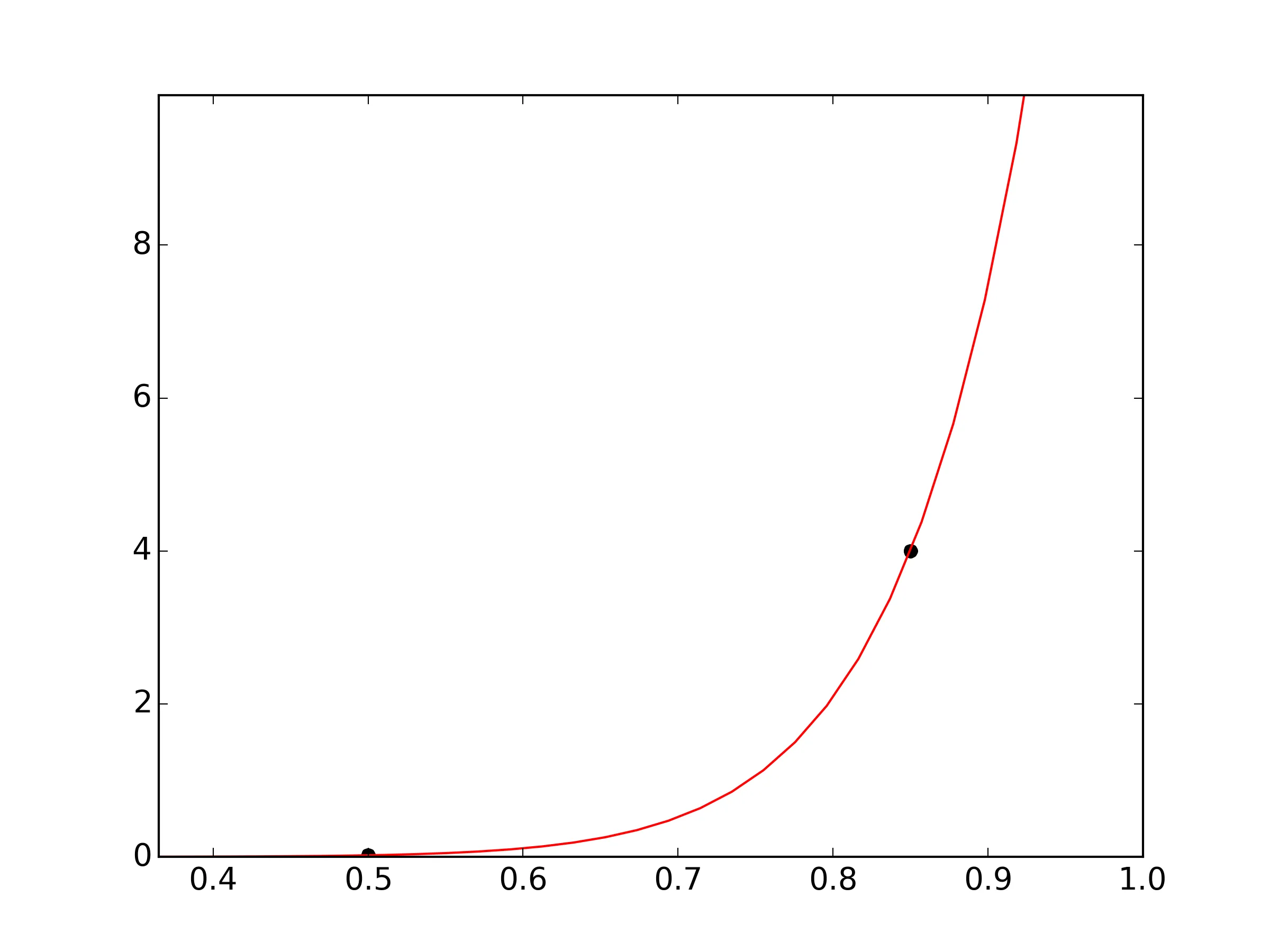
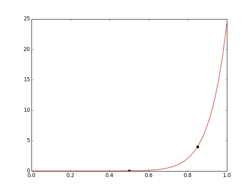
我想用指数函数 y=x ** pw，其中pw是常数，使其通过两个数据点。使用scipy中的 curve_fit 函数可以优化adj1和adj2。我已经尝试了下面的代码但无法让它正常工作。曲线没有经过数据点。如何修复它？

import numpy as np
import matplotlib.pyplot as plt
from scipy.optimize import curve_fit

def func(x, adj1,adj2):
    return np.round(((x+adj1) ** pw) * adj2, 2)

x = [0.5,0.85] # two given datapoints to which the exponential function with power pw should fit
y = [0.02,4]

pw=15
popt, pcov = curve_fit(func, x, y)

xf=np.linspace(0,1,50)

plt.figure()
plt.plot(x, y, 'ko', label="Original Data")
plt.plot(xf, func(xf, *popt), 'r-', label="Fitted Curve")
plt.show()

- Nickpick

Answer 1

如果你想从仅有的两个数据点中找到目标函数中的两个参数，对于最小二乘拟合来说并不是问题：只需要解出同时方程 y1 = b(x1+a)^p 和 y2 = b(x2+a)^p 中的参数 a 和 b。

import numpy as np
import matplotlib.pyplot as plt

def func(x, adj1,adj2):
    return ((x+adj1) ** pw) * adj2

x = [0.5,0.85] # two given datapoints to which the exponential function with power pw should fit
y = [0.02,4]

pw = 15
A = np.exp(np.log(y[0]/y[1])/pw)
a = (x[0] - x[1]*A)/(A-1)
b = y[0]/(x[0]+a)**pw

xf=np.linspace(0,1,50)
plt.figure()
plt.plot(x, y, 'ko', label="Original Data")
plt.plot(xf, func(xf, a, b), 'r-', label="Fitted Curve")
plt.show()

生成的函数将确切地穿过这两个点。

- xnx

---

我同意。Scipy唯一的问题是您无法将函数的某些参数保持为常量。 - Nickpick

Answer 2

这是因为 round 方法破坏了 curve_fit 搜索空间的能力。对 p0 的微小扰动总会得到相同的结果，因此它立即停止搜索，并始终返回您提供的起始点（默认为 p0 = [1.,1.]）。解决方法是从函数中简单地删除 np.round。

import numpy as np
import matplotlib.pyplot as plt
from scipy.optimize import curve_fit

def func(x, adj1,adj2):
    return ((x+adj1) ** pw) * adj2

x = [0.5,0.85] # two given datapoints to which the exponential function with power pw should fit
y = [0.02,4]

pw=15
popt, pcov = curve_fit(func, x, y)

xf=np.linspace(0,1,50)

plt.figure()
plt.plot(x, y, 'ko', label="Original Data")
plt.plot(xf, func(xf, *popt), 'r-', label="Fitted Curve")
plt.show()

- joshua

Answer 3

这里是解决方案。我认为在曲线拟合方面，lmfit是scipy的一个很好的替代品。

from lmfit import minimize, Parameters, Parameter, report_fit
import numpy as np

# create data to be fitted
xf = [0.5,0.85] # two given datapoints to which the exponential function with power pw should fit
yf = [0.02,4]

# define objective function: returns the array to be minimized
def fcn2min(params, x, data):
    pw = params['pw'].value
    adj1 = params['adj1'].value
    adj2 = params['adj2'].value

    model = adj1 * np.power(x + adj2, pw)
    return model - data

pw=2

# create a set of Parameters
params = Parameters()
params.add('pw',   value= pw, vary=False)
params.add('adj1', value= 1)
params.add('adj2', value= 1)


# do fit, here with leastsq model
result = minimize(fcn2min, params, args=(xf, yf))

# calculate final result
final = yf + result.residual

# write error report
report_fit(result.params)
adj1=result.params['adj1']
adj2=result.params['adj2']

# try to plot results
x = np.linspace(0, 1, 100)
y = adj1 * np.power(x + adj2, pw)

import pylab
pylab.plot(xf, yf, 'ko')
pylab.plot(x, y, 'r')
pylab.show()

- Nickpick

---

lmfit是一个非常棒的工具，在一些scipy失败的情况下（有界或约束局部求解器）也能够正常工作。 - Moritz