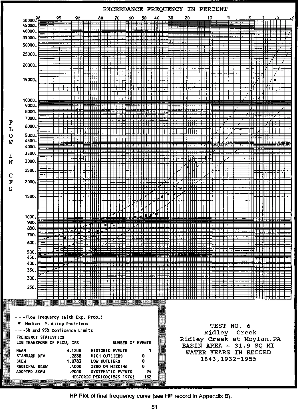
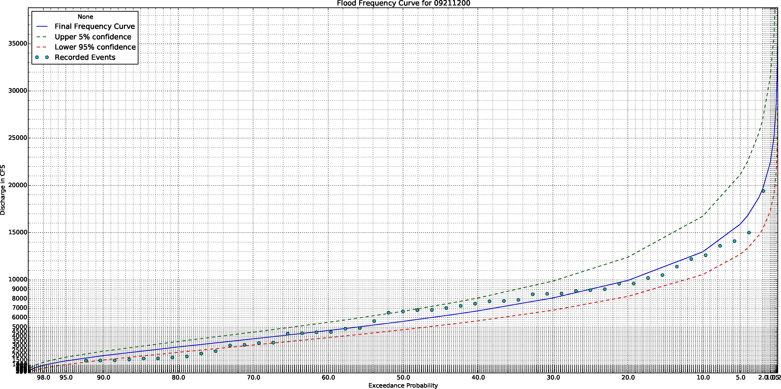
多亏了@Amy Teegarden的帮助,我终于得出了正确的解决方案。为了让其他人参考,我想在这里分享最终的解决方案!以下是最终结果:
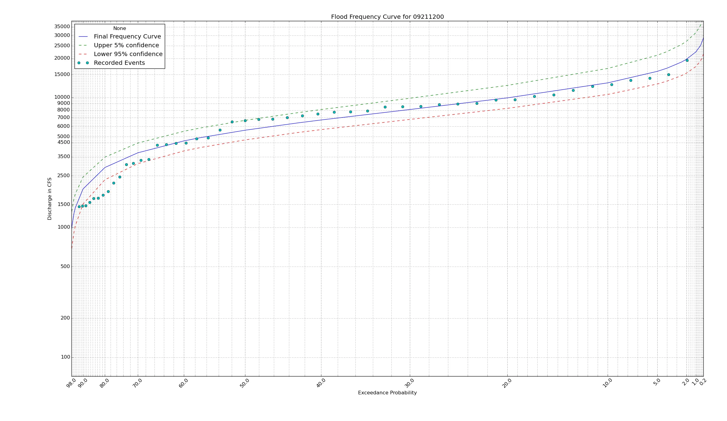
下面是一个真正的概率轴比例尺,使用正态累积分布函数和其反函数PPF,参数化为mu和sigma。
import numpy as np
from matplotlib import scale as mscale
from matplotlib import transforms as mtransforms
from matplotlib.ticker import FormatStrFormatter, FixedLocator
from scipy.stats import norm
class ProbScale(mscale.ScaleBase):
"""
Scales data in range 0 to 100 using a non-standard log transform
This scale attempts to replicate "probability paper" scaling
The scale function:
A piecewise combination of exponential, linear, and logarithmic scales
The inverse scale function:
piecewise combination of exponential, linear, and logarithmic scales
Since probabilities at 0 and 100 are not represented,
there is user-defined upper and lower limit, above and below which nothing
will be plotted. This defaults to .1 and 99 for lower and upper, respectively.
"""
name = 'prob_scale'
def __init__(self, axis, **kwargs):
"""
Any keyword arguments passed to ``set_xscale`` and
``set_yscale`` will be passed along to the scale's
constructor.
upper: The probability above which to crop the data.
lower: The probability below which to crop the data.
"""
mscale.ScaleBase.__init__(self)
upper = kwargs.pop("upper", 98)
if upper <= 0 or upper >= 100:
raise ValueError("upper must be between 0 and 100.")
lower = kwargs.pop("lower", 0.2)
if lower <= 0 or lower >= 100:
raise ValueError("lower must be between 0 and 100.")
if lower >= upper:
raise ValueError("lower must be strictly less than upper!.")
self.lower = lower
self.upper = upper
mu = kwargs.pop("mu", 15)
sigma = kwargs.pop("sigma", 40)
self.mu = mu
self.sigma = sigma
axis.axes.set_xlim(lower,upper)
def get_transform(self):
"""
Override this method to return a new instance that does the
actual transformation of the data.
The ProbTransform class is defined below as a
nested class of this one.
"""
return self.ProbTransform(self.lower, self.upper, self.mu, self.sigma)
def set_default_locators_and_formatters(self, axis):
"""
Override to set up the locators and formatters to use with the
scale. This is only required if the scale requires custom
locators and formatters. Writing custom locators and
formatters: many helpful examples in ``ticker.py``.
In this case, the prob_scale uses a fixed locator from
0.1 to 99 % and a custom no formatter class
This builds both the major and minor locators, and cuts off any values
above or below the user defined thresholds: upper, lower
"""
major_ticks = np.asarray([.2,1,2,5,10,20,30,40,50,60,70,80,90,98])
major_ticks = major_ticks[np.where( (major_ticks >= self.lower) & (major_ticks <= self.upper) )]
minor_ticks = np.concatenate( [np.arange(.2, 1, .1), np.arange(1, 2, .2), np.arange(2,20,1), np.arange(20, 80, 2), np.arange(80, 98, 1)] )
minor_ticks = minor_ticks[np.where( (minor_ticks >= self.lower) & (minor_ticks <= self.upper) )]
axis.set_major_locator(FixedLocator(major_ticks))
axis.set_minor_locator(FixedLocator(minor_ticks))
def limit_range_for_scale(self, vmin, vmax, minpos):
"""
Override to limit the bounds of the axis to the domain of the
transform. In the case of Probability, the bounds should be
limited to the user bounds that were passed in. Unlike the
autoscaling provided by the tick locators, this range limiting
will always be adhered to, whether the axis range is set
manually, determined automatically or changed through panning
and zooming.
"""
return max(self.lower, vmin), min(self.upper, vmax)
class ProbTransform(mtransforms.Transform):
input_dims = 1
output_dims = 1
is_separable = True
def __init__(self, upper, lower, mu, sigma):
mtransforms.Transform.__init__(self)
self.upper = upper
self.lower = lower
self.mu = mu
self.sigma = sigma
def transform_non_affine(self, a):
"""
This transform takes an Nx1 ``numpy`` array and returns a
transformed copy. Since the range of the Probability scale
is limited by the user-specified threshold, the input
array must be masked to contain only valid values.
``matplotlib`` will handle masked arrays and remove the
out-of-range data from the plot. Importantly, the
``transform`` method *must* return an array that is the
same shape as the input array, since these values need to
remain synchronized with values in the other dimension.
"""
masked = np.ma.masked_where( (a < self.upper) & (a > self.lower) , a)
cdf = norm.cdf(masked, self.mu, self.sigma)*100
return cdf
def inverted(self):
"""
Override this method so matplotlib knows how to get the
inverse transform for this transform.
"""
return ProbScale.InvertedProbTransform(self.lower, self.upper, self.mu, self.sigma)
class InvertedProbTransform(mtransforms.Transform):
input_dims = 1
output_dims = 1
is_separable = True
def __init__(self, lower, upper, mu, sigma):
mtransforms.Transform.__init__(self)
self.lower = lower
self.upper = upper
self.mu = mu
self.sigma = sigma
def transform_non_affine(self, a):
inverse = norm.ppf(a/100, self.mu, self.sigma)
return inverse
def inverted(self):
return ProbScale.ProbTransform(self.lower, self.upper)
mscale.register_scale(ProbScale)
另外,为了获得所需的y轴结果,我发现对数刻度确实可以使用一些额外的调整来获得合理的图形。以下是用于强制对数刻度具有适当次要刻度的代码:
axes.set_yscale('log', basey=10, subsy=[2,3,4,5,6,7,8,9])
然后,您可以使用定位器和格式化程序修改标签:
axes.yaxis.set_minor_locator(FixedLocator([200, 500, 1500, 2500, 3500, 4500, 5000, 6000, 7000, 8000, 9000, 15000, 20000, 25000, 30000, 35000, 40000, 45000, 50000]))
axes.yaxis.set_minor_formatter(FormatStrFormatter('%d'))
axes.yaxis.set_major_formatter(FormatStrFormatter('%d'))
所以完整的轴操作如下所示:
axes.set_ylabel('Discharge in CFS')
axes.set_xlabel('Exceedance Probability')
plt.setp(plt.xticks()[1], rotation=45)
axes.set_yscale('log', basey=10, subsy=[2,3,4,5,6,7,8,9])
axes.set_xscale('prob_scale', upper=98, lower=.2)
axes.yaxis.set_minor_locator(FixedLocator([200, 500, 1500, 2500, 3500, 4500, 5000, 6000, 7000, 8000, 9000, 15000, 20000, 25000, 30000, 35000, 40000, 45000, 50000]))
axes.yaxis.set_minor_formatter(FormatStrFormatter('%d'))
axes.yaxis.set_major_formatter(FormatStrFormatter('%d'))
axes.set_ylim((0, 2*pp['Q'].max()))
axes.invert_xaxis()
axes.grid(which='both', alpha=.9)
这提供了一个半对数概率纸图!其良好特性是任何绘制在这些轴上的东西,如果呈直线状,则表明它来自正态分布!