如何使用matplotlib绘制复数(阿甘图)

1
我不确定你在寻求什么......如果你有一组复数,并想通过使用它们的实部作为x坐标和虚部作为y坐标将它们映射到平面上,那么您可以使用 number.real 获取任何Python虚数的实部,使用number.imag获取虚部。如果你使用numpy,它还提供了一组辅助函数,如numpy.real和numpy.imag等,可用于numpy数组。
例如,如果你有一个存储在数组中的复数,像这样:
In [13]: a = n.arange(5) + 1j*n.arange(6,11)

In [14]: a
Out[14]: array([ 0. +6.j,  1. +7.j,  2. +8.j,  3. +9.j,  4.+10.j])
...你只需做
In [15]: fig,ax = subplots()

In [16]: ax.scatter(a.real,a.imag)
这将在Argand图中为每个点绘制点。
编辑:对于绘图部分,你当然必须通过from matplotlib.pyplot import *导入matplotlib.pyplot或者(像我一样)使用ipython shell处于pylab模式。
1
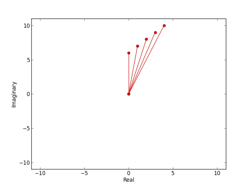
关于@inclement的回答,以下函数生成一个以0,0为中心、按一组复数中的最大绝对值进行缩放的阿根廷图。
我使用了plot函数并指定了从(0,0)开始的实线。通过用ro替换ro-可以去除这些实线。
def argand(a):
    import matplotlib.pyplot as plt
    import numpy as np
    for x in range(len(a)):
        plt.plot([0,a[x].real],[0,a[x].imag],'ro-',label='python')
    limit=np.max(np.ceil(np.absolute(a))) # set limits for axis
    plt.xlim((-limit,limit))
    plt.ylim((-limit,limit))
    plt.ylabel('Imaginary')
    plt.xlabel('Real')
    plt.show()
>>> a = n.arange(5) + 1j*n.arange(6,11)
>>> from argand import argand
>>> argand(a)
产生:
编辑:
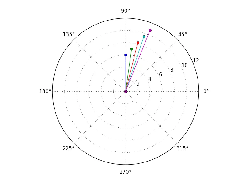
我刚刚意识到还有一个polar绘图函数:
for x in a:
    plt.polar([0,angle(x)],[0,abs(x)],marker='o')
2
label = 'python'是什么意思? - lpnorm如果你喜欢下面这样的图表:
或者这样的图表:第二种类型的图表
你可以通过以下两行代码轻松实现(以上面的图表为例):
z=[20+10j,15,-10-10j,5+15j] # array of complex values

complex_plane2(z,1) # function to be called
通过使用此处的简单Jupyter代码https://github.com/osnove/other/blob/master/complex_plane.py
我编写它是为了自己的目的。如果它能帮助其他人,那就更好了。
1
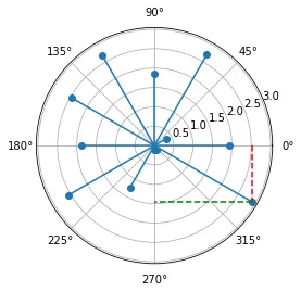
cmath.polar 将一个复数转换为极坐标rho-theta坐标系。在下面的代码中,首先对此函数进行了矢量化,以处理复数数组而不是单个数字,这只是为了防止使用显式循环。
将
pyplot轴与其投影类型设置为polar。可以使用pyplot.stem或pyplot.scatter进行绘制。
为了绘制笛卡尔坐标系的水平和垂直线,有两种可能性:
添加笛卡尔坐标轴并绘制笛卡尔坐标。该解决方案在this question中描述。我认为这不是一个简单的解决方案,因为笛卡尔坐标轴不会居中,也不会有正确的比例因子。
使用极轴,并将笛卡尔坐标转换为极坐标进行投影。这是我用来绘制上面图形的解决方案。为了不使图形杂乱无章,我只显示了一个点及其投影的笛卡尔坐标。
用于上图的代码:
from cmath import pi, e, polar
from numpy import linspace, vectorize, sin, cos
from numpy.random import rand
from matplotlib import pyplot as plt

# Arrays of evenly spaced angles, and random lengths
angles = linspace(0, 2*pi, 12, endpoint=False)
lengths = 3*rand(*angles.shape)

# Create an array of complex numbers in Cartesian form
z = lengths * e ** (1j*angles)

# Convert back to polar form
vect_polar = vectorize(polar)
rho_theta = vect_polar(z)

# Plot numbers on polar projection
fig, ax = plt.subplots(subplot_kw={'projection': 'polar'})
ax.stem(rho_theta[1], rho_theta[0])

# Get a number, find projections on axes
n = 11
rho, theta = rho_theta[0][n], rho_theta[1][n]
a = cos(theta)
b = sin(theta)
rho_h, theta_h = abs(a)*rho, 0 if a >= 0 else -pi
rho_v, theta_v = abs(b)*rho, pi/2 if b >= 0 else -pi/2

# Plot h/v lines on polar projection
ax.plot((theta_h, theta), (rho_h, rho), c='r', ls='--')
ax.plot((theta, theta_v), (rho, rho_v), c='g', ls='--')
import matplotlib.pyplot as plt
from numpy import *


'''
~~~~~~~~~~~~~~~~~~~~~~~~~~~~~~~~~~~`
This draws the axis for argand diagram
~~~~~~~~~~~~~~~~~~~~~~~~~~~~~~~~~~~`
'''
r = 1
Y = [r*exp(1j*theta) for theta in linspace(0,2*pi, 200)]
Y = array(Y)
plt.plot(real(Y), imag(Y), 'r')
plt.ylabel('Imaginary')
plt.xlabel('Real')
plt.axhline(y=0,color='black')
plt.axvline(x=0, color='black')


def argand(complex_number):
    '''
    This function takes a complex number.
    '''
    y = complex_number
    x1,y1 = [0,real(y)], [0, imag(y)]
    x2,y2 = [real(y), real(y)], [0, imag(y)]


    plt.plot(x1,y1, 'r') # Draw the hypotenuse
    plt.plot(x2,y2, 'r') # Draw the projection on real-axis

    plt.plot(real(y), imag(y), 'bo')

[argand(r*exp(1j*theta)) for theta in linspace(0,2*pi,100)]
plt.show()
https://github.com/QuantumNovice/Matplotlib-Argand-Diagram/blob/master/argand.py
原文链接