有没有办法在ggmap中添加一个比例尺(用于线性距离)?

19

虽然这并不是我的问题所必需的内容,但这里是我的绘图示例,我想在其上添加比例尺。

ggmap(get_map(location = "Kinston, NC", zoom = 12, maptype = 'hybrid')) +
geom_point(x = -77.61198, y = 35.227792, colour = "red", size = 5) +
geom_point(x = -77.57306, y = 35.30288, colour = "blue", size = 3) +
geom_point(x = -77.543, y = 35.196, colour = "blue", size = 3) +
geom_text(x = -77.575, y = 35.297, label = "CRONOS Data") +
geom_text(x = -77.54, y = 35.19, label = "NOAA") +
geom_text(x = -77.61, y = 35.22, label = "PP Site")

北卡罗来纳地图


嗨,请查看?OSM_scale_lookup和相关的FAQ链接。 - Ricardo Saporta
Oswaldo Santos的ggsn包可以为使用ggplot或ggmap创建的地图添加比例尺。此外,您还可以查看stackoverflow中提出的其他类似问题的解决方案。 - josep maria porrà
2个回答

17

要实现这一点,您需要完成几个步骤。

第一步是将您的数据放入一个data.frame()中:

sites.data = data.frame(lon = c(-77.61198, -77.57306, -77.543),
                        lat = c(35.227792, 35.30288, 35.196),
                        label = c("PP Site","NOAA", "CRONOS Data"),
                        colour = c("red","blue","blue"))

现在我们可以使用 gg_map 包获取该地区的地图:

require(gg_map)
map.base <- get_map(location = c(lon = mean(sites.data$lon),
                                 lat = mean(sites.data$lat)),
                    zoom = 10) # could also use zoom = "auto"

我们需要那张图片的尺寸:

bb <- attr(map.base,"bb")

现在我们开始确定比例尺。首先,我们需要一个函数,根据纬度/经度给出两点之间的距离。为此,我们使用Haversine公式,由Floris在计算两个GPS点之间(x,y)距离中描述:

distHaversine <- function(long, lat){

  long <- long*pi/180
  lat <- lat*pi/180  
  dlong = (long[2] - long[1])
  dlat  = (lat[2] - lat[1])

  # Haversine formula:
  R = 6371;
  a = sin(dlat/2)*sin(dlat/2) + cos(lat[1])*cos(lat[2])*sin(dlong/2)*sin(dlong/2)
  c = 2 * atan2( sqrt(a), sqrt(1-a) )
  d = R * c
  return(d) # in km
}
下一步是确定定义比例尺的点。在这个例子中,我把东西放在了图的左下角,使用我们已经找出的边界框:
sbar <- data.frame(lon.start = c(bb$ll.lon + 0.1*(bb$ur.lon - bb$ll.lon)),
                   lon.end = c(bb$ll.lon + 0.25*(bb$ur.lon - bb$ll.lon)),
                   lat.start = c(bb$ll.lat + 0.1*(bb$ur.lat - bb$ll.lat)),
                   lat.end = c(bb$ll.lat + 0.1*(bb$ur.lat - bb$ll.lat)))

sbar$distance = distHaversine(long = c(sbar$lon.start,sbar$lon.end),
                              lat = c(sbar$lat.start,sbar$lat.end))

最后,我们可以使用比例尺绘制地图。

ptspermm <- 2.83464567  # need this because geom_text uses mm, and themes use pts. Urgh.

map.scale <- ggmap(map.base,
                   extent = "normal", 
                   maprange = FALSE) %+% sites.data +
  geom_point(aes(x = lon,
                 y = lat,
                 colour = colour)) +
  geom_text(aes(x = lon,
                y = lat,
                label = label),
            hjust = 0,
            vjust = 0.5,
            size = 8/ptspermm) +    
  geom_segment(data = sbar,
               aes(x = lon.start,
                   xend = lon.end,
                   y = lat.start,
                   yend = lat.end)) +
  geom_text(data = sbar,
            aes(x = (lon.start + lon.end)/2,
           y = lat.start + 0.025*(bb$ur.lat - bb$ll.lat),
           label = paste(format(distance, 
                                digits = 4,
                                nsmall = 2),
                         'km')),
           hjust = 0.5,
           vjust = 0,
           size = 8/ptspermm)  +
  coord_map(projection="mercator",
            xlim=c(bb$ll.lon, bb$ur.lon),
            ylim=c(bb$ll.lat, bb$ur.lat))  

然后我们保存它...

# Fix presentation ----
map.out <- map.scale +  
  theme_bw(base_size = 8) +
  theme(legend.justification=c(1,1), 
        legend.position = c(1,1)) 

ggsave(filename ="map.png", 
       plot = map.out,
       dpi = 300,
       width = 4, 
       height = 3,
       units = c("in"))

这将使你得到类似于以下的东西:

带有比例尺的地图

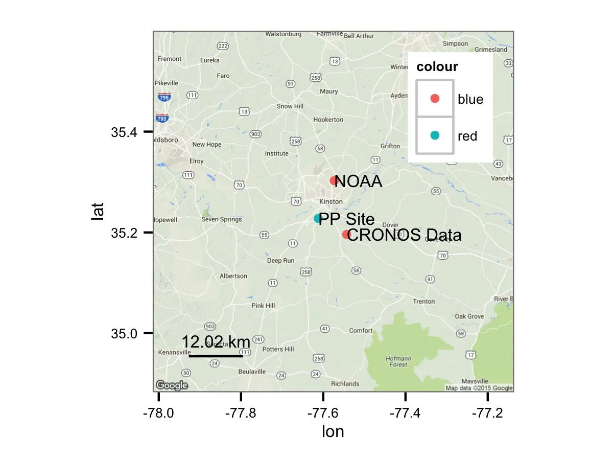
好处在于所有的绘图都使用ggplot2(),因此您可以使用http://ggplot2.org上的文档,使其看起来符合您的需求。


这是一个非常有帮助的答案,@AndyClifton! - Mikko
我正在尝试使用你的代码,但不确定是否存在错误?在这里双重检查你的经纬度示例:[链接](http://www.movable-type.co.uk/scripts/latlong.html)得到的结果是12.02公里,而不是你的公式得到的13.52公里? - maja zaloznik
1
更新于2015年11月30日,修复了@maja注意到的问题,这是由于我在距离计算中未将纬度/经度表达为弧度所导致的。 - Andy Clifton

8
我重新处理了@Andy Clifton的代码,增加了更精确的距离测量,并允许比例尺具有所需的长度,而不是依赖于比例尺的位置。虽然我找不到错误,但Andy的代码已经帮助我解决了99%的问题,但他代码中使用的Haversine公式未经其他来源验证。
这个第一部分只是为了完整性将从Andy Clifton的答案复制过来的代码:
sites.data = data.frame(lon = c(-77.61198, -77.57306, -77.543),
                        lat = c(35.227792, 35.30288, 35.196),
                        label = c("PP Site","NOAA", "CRONOS Data"),
                        colour = c("red","blue","blue"))
map.base <- get_map(location = c(lon = mean(sites.data$lon),
                                   lat = mean(sites.data$lat)),
                      zoom = 10)
bb <- attr(map.base,"bb")
sbar <- data.frame(lon.start = c(bb$ll.lon + 0.1*(bb$ur.lon - bb$ll.lon)),
                     lon.end = c(bb$ll.lon + 0.25*(bb$ur.lon - bb$ll.lon)),
                     lat.start = c(bb$ll.lat + 0.1*(bb$ur.lat - bb$ll.lat)),
                     lat.end = c(bb$ll.lat + 0.1*(bb$ur.lat - bb$ll.lat)))

下面的两个步骤是不同的:
首先,使用“geosphere”包中的“distVincentyEllipsoid”函数来计算距离,比Haversine公式更加精确:
sbar$distance <- geosphere::distVincentyEllipsoid(c(sbar$lon.start,sbar$lat.start),
 c(sbar$lon.end,sbar$lat.end))

然后,根据您的地图比例尺,将比例尺校正为标准长度。在本例中,20公里似乎是一个不错的合理选择,即20,000米:

scalebar.length <- 20
sbar$lon.end <- sbar$lon.start +
((sbar$lon.end-sbar$lon.start)/sbar$distance)*scalebar.length*1000

我只是在Andy的代码中添加了箭头到geom_segment,因为我认为这样看起来更好看。

ptspermm <- 2.83464567  # need this because geom_text uses mm, and themes use pts. Urgh.

map.scale <- ggmap(map.base,
                   extent = "normal", 
                   maprange = FALSE) %+% sites.data +
  geom_point(aes(x = lon,
                 y = lat,
                 colour = colour)) +
  geom_text(aes(x = lon,
                y = lat,
                label = label),
            hjust = 0,
            vjust = 0.5,
            size = 8/ptspermm) +    
  geom_segment(data = sbar,
               aes(x = lon.start,
                   xend = lon.end,
                   y = lat.start,
                   yend = lat.end),
               arrow=arrow(angle = 90, length = unit(0.1, "cm"),
                           ends = "both", type = "open")) +
  geom_text(data = sbar,
            aes(x = (lon.start + lon.end)/2,
                y = lat.start + 0.025*(bb$ur.lat - bb$ll.lat),
                label = paste(format(scalebar.length),
                              'km')),
            hjust = 0.5,
            vjust = 0,
            size = 8/ptspermm)  +
  coord_map(projection = "mercator",
            xlim=c(bb$ll.lon, bb$ur.lon),
            ylim=c(bb$ll.lat, bb$ur.lat))  

# Fix presentation ----
map.out <- map.scale +  
  theme_bw(base_size = 8) +
  theme(legend.justification = c(1,1), 
        legend.position = c(1,1)) 

ggsave(filename ="map.png", 
       plot = map.out,
       dpi = 300,
       width = 4, 
       height = 3,
       units = c("in"))

reworked scale bar example


网页内容由stack overflow 提供, 点击上面的
可以查看英文原文,
原文链接