指定
interval 和
level 参数时,
predict.lm 可以返回置信区间(CI)或预测区间(PI)。本答案展示如何在不设置这些参数的情况下获得 CI 和 PI。有两种方法:
- 使用来自
predict.lm 的中间结果;
- 从头开始做。
了解如何使用这两种方式可以全面了解预测过程。
请注意,我们仅涵盖
predict.lm 的默认情况下的
type =“response”。讨论
type =“terms” 超出了本答案的范围。
设置
为了帮助其他读者复制、粘贴和运行代码,我在此收集您的代码。我还更改了变量名称,使它们具有更清晰的含义。此外,我扩展了
newdat 来包括多个行,以显示我们的计算是“向量化”的。
dat <- structure(list(V1 = c(20L, 60L, 46L, 41L, 12L, 137L, 68L, 89L,
          4L, 32L, 144L, 156L, 93L, 36L, 72L, 100L, 105L, 131L, 127L, 57L,
          66L, 101L, 109L, 74L, 134L, 112L, 18L, 73L, 111L, 96L, 123L,
          90L, 20L, 28L, 3L, 57L, 86L, 132L, 112L, 27L, 131L, 34L, 27L,
          61L, 77L), V2 = c(2L, 4L, 3L, 2L, 1L, 10L, 5L, 5L, 1L, 2L, 9L,
          10L, 6L, 3L, 4L, 8L, 7L, 8L, 10L, 4L, 5L, 7L, 7L, 5L, 9L, 7L,
          2L, 5L, 7L, 6L, 8L, 5L, 2L, 2L, 1L, 4L, 5L, 9L, 7L, 1L, 9L, 2L,
          2L, 4L, 5L)), .Names = c("V1", "V2"),
          class = "data.frame", row.names = c(NA, -45L))

lmObject <- lm(V1 ~ V2, data = dat)

newdat <- data.frame(V2 = c(6, 7))
以下是
predict.lm的输出结果,稍后将与我们的手动计算进行比较。
predict(lmObject, newdat, se.fit = TRUE, interval = "confidence", level = 0.90)
predict(lmObject, newdat, se.fit = TRUE, interval = "prediction", level = 0.90)
使用predict.lm的中间结果
z <- predict(lmObject, newdat, se.fit = TRUE)
se.fit是什么?
z$se.fit是预测均值z$fit的标准误差,用于构建z$fit的置信区间。我们还需要自由度为z$df的t分布的分位数。
alpha <- 0.90
Qt <- c(-1, 1) * qt((1 - alpha) / 2, z$df, lower.tail = FALSE)
CI <- z$fit + outer(z$se.fit, Qt)
colnames(CI) <- c("lwr", "upr")
CI
我们可以看到,这与
predict.lm(, interval = "confidence")相符。
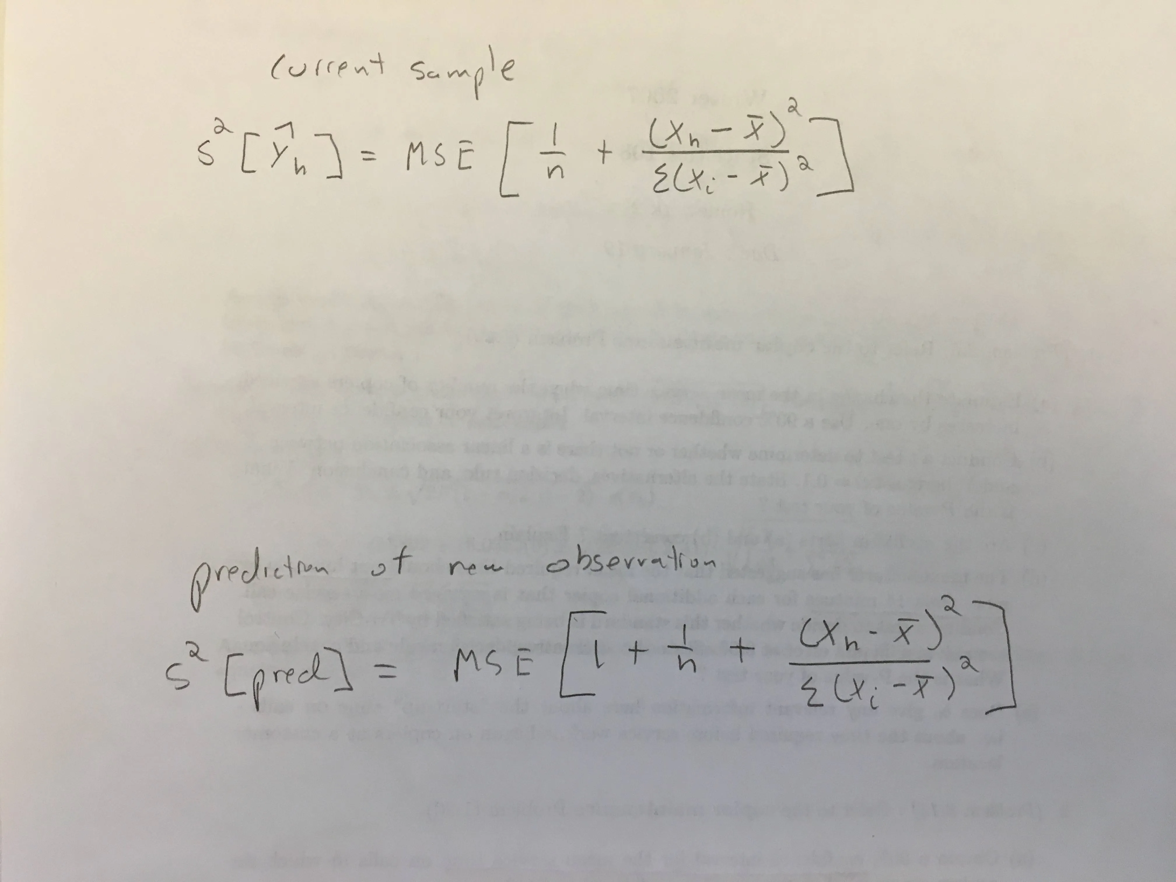
PI的标准误差是多少?
PI比CI更宽,因为它考虑了残差方差:
variance_of_PI = variance_of_CI + variance_of_residual
请注意,这是逐点定义的。对于非加权线性回归(如您的示例),残差方差在各处相等(称为同方差性),它是 z$residual.scale ^ 2。因此,PI 的标准误差为:
se.PI <- sqrt(z$se.fit ^ 2 + z$residual.scale ^ 2)
PI是这样构建的
PI <- z$fit + outer(se.PI, Qt)
colnames(PI) <- c("lwr", "upr")
PI
我们可以看到这与 predict.lm(, interval = "prediction") 相符。
备注
如果您使用加权线性回归,情况会更加复杂,因为残差方差不是均等的,所以应该加权 z$residual.scale ^ 2。对于拟合值(即在使用 predict.lm 中的 type = "prediction" 时不设置 newdata),构建 PI 更容易,因为权重已知(在使用 lm 时必须通过 weight 参数提供)。对于外部预测(即将 newdata 传递给 predict.lm),predict.lm 希望您告诉它如何加权残差方差。您需要在 predict.lm 中使用参数 pred.var 或 weights,否则您将收到来自 predict.lm 的警告,提示无法构建 PI 的信息不足。以下内容摘自 ?predict.lm:
 The prediction intervals are for a single observation at each case
 in ‘newdata’ (or by default, the data used for the fit) with error
 variance(s) ‘pred.var’.  This can be a multiple of ‘res.var’, the
 estimated value of sigma^2: the default is to assume that future
 observations have the same error variance as those used for
 fitting.  If ‘weights’ is supplied, the inverse of this is used as
 a scale factor.  For a weighted fit, if the prediction is for the
 original data frame, ‘weights’ defaults to the weights used for
 the model fit, with a warning since it might not be the intended
 result.  If the fit was weighted and ‘newdata’ is given, the
 default is to assume constant prediction variance, with a warning.
请注意,CI的构建不受回归类型影响。
从头开始做一切
基本上,我们想知道如何在z中获取fit、se.fit、df和residual.scale。
预测均值可以通过矩阵向量乘法Xp %*% b计算,其中Xp是线性预测矩阵,b是回归系数向量。
Xp <- model.matrix(delete.response(terms(lmObject)), newdat)
b <- coef(lmObject)
yh <- c(Xp %*% b)
我们可以看到这与z$fit相符。 yh的方差协方差为Xp %*% V %*% t(Xp),其中V是b的方差协方差矩阵,可以通过以下方式计算:
V <- vcov(lmObject)
yh的完整方差-协方差矩阵不需要计算点估计的CI或PI。我们只需要它的主对角线。因此,我们可以通过以下更有效的方式进行而不是执行
diag(Xp %*% V %*% t(Xp)):
var.fit <- rowSums((Xp %*% V) * Xp)
sqrt(var.fit)
剩余自由度在拟合模型中很容易获得:
dof <- df.residual(lmObject)
#[1] 43
最后,为计算残差方差,请使用Pearson估计量:
sig2 <- c(crossprod(lmObject$residuals)) / dof
sqrt(sig2)
注意
在加权回归的情况下,应按以下方式计算sig2:
sig2 <- c(crossprod(sqrt(lmObject$weights) * lmObject$residuals)) / dof
附录:自编函数模仿 predict.lm
"从头开始做一切"中的代码已经整理成一个函数lm_predict,请参考这个问答:使用线性模型lm:如何获得预测值总和的预测方差。
?predict.lm,它说:*"se.fit: 预测均值的标准误差"。* "预测均值"听起来好像只适用于置信区间。如果你不想看到它,可以将se.fit = FALSE。 - Gregor Thomas