对于一个没有任何努力的“为我编写这段代码”的问题,你确实有很多具体的要求。虽然这不符合你的标准,但也许对于使用基本图形的某些人会有用。
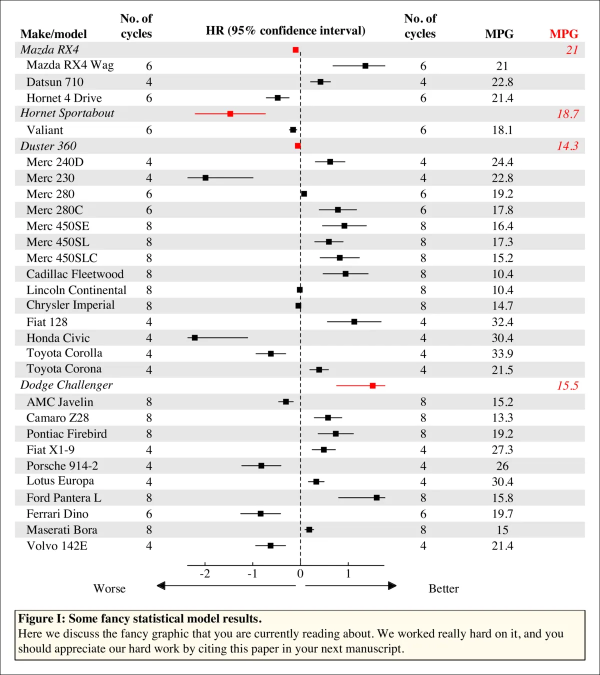
中间面板中的情节可以是任何东西,只要每行有一个情节,并且在其中有点匹配即可。(实际上这并不正确,如果您想要,任何类型的情节都可以放在该面板中,因为它只是一个普通的绘图窗口)。此代码中有三个示例:点、箱线图和线条。

这是输入数据。只是一个通用列表和“标题”的索引,我认为比“直接使用回归对象”要好得多。
## indices of headers
idx <- c(1,5,7,22)
l <- list('Make/model' = rownames(mtcars),
          'No. of\ncycles' = mtcars$cyl,
          MPG = mtcars$mpg)
l[] <- lapply(seq_along(l), function(x)
  ifelse(seq_along(l[[x]]) %in% idx, l[[x]], paste0('  ', l[[x]])))

# List of 3
#  $ Make/model    : chr [1:32] "Mazda RX4" "  Mazda RX4 Wag" "  Datsun 710" "  Hornet 4 Drive" ...
#  $ No. of
# cycles: chr [1:32] "6" "  6" "  4" "  6" ...
#  $ MPG           : chr [1:32] "21" "  21" "  22.8" "  21.4" ...
我意识到这段代码生成了一个PDF。我不想将其转换为图像上传,所以我用imagemagick将其转换了。
pl <- c('point','box','line')[1]
pad <- c(0,0,0,0)
oma <- c(1,1,2,1)
xfig = c(.25,.45,.3)
yfig = c(.15, .85)
cairo_pdf('~/desktop/pl.pdf', height = 9, width = 8)
x <- l[-3]
lx <- seq_along(x[[1]])
nx <- length(lx)
xcf <- cumsum(xfig)[-length(xfig)]
ycf <- cumsum(yfig)[-length(yfig)]
plot.new()
par(oma = oma, mar = c(0,0,0,0), family = 'serif')
plot.window(range(seq_along(x)), range(lx))
par(fig = c(0,1,ycf,1), oma = par('oma') + pad)
bars(lx)
par(fig = c(0,1,0,ycf), mar = c(0,0,3,0), oma = oma + pad)
p <- par('usr')
box('plot')
rect(p[1], p[3], p[2], p[4], col = adjustcolor('cornsilk', .5))
mtext('\tFigure I: Some fancy statistical model results.',
adj = 0, font = 2, line = -1)
mtext(paste('\tHere we discuss the fancy graphic that you are currently reading',
'about. We worked really hard on it, and you\n\tshould appreciate',
'our hard work by citing this paper in your next manuscript.'),
adj = 0, line = -3)
lp <- l[1:2]
par(fig = c(0,xcf[1],ycf,1), oma = oma + vec(pad, 0, 4))
plot_text(lp, c(1,2),
adj = rep(0:1, c(nx, nx)),
font = vec(1, 3, idx, nx),
col = c(rep(1, nx), vec(1, 'transparent', idx, nx))
) -> at
vtext(unique(at$x), max(at$y) + c(1,1.5), names(lp),
font = 2, xpd = NA, adj = c(0,1))
rp <- l[c(2:3,3)]
par(fig = c(tail(xcf, -1),1,ycf,1), oma = oma + vec(pad, 0, 2))
plot_text(rp, c(1,2),
col = c(rep(vec(1, 'transparent', idx, nx), 2),
vec('transparent', 2, idx, nx)),
font = vec(1, 3, idx, nx),
adj = rep(c(NA,NA,1), each = nx)
) -> at
vtext(unique(at$x), max(at$y) + c(1.5,1,1), names(rp),
font = 2, xpd = NA, adj = c(NA, NA, 1), col = c(1,1,2))
par(new = TRUE, fig = c(xcf[1], xcf[2], ycf, 1),
mar = c(0,2,0,2), oma = oma + vec(pad, 0, c(2,4)))
set.seed(1)
xx <- rev(rnorm(length(lx)))
yy <- rev(lx)
plot(xx, yy, ann = FALSE, axes = FALSE, type = 'n',
panel.first = {
segments(0, 0, 0, nx, lty = 'dashed')
},
panel.last = {
if (pl == 'point') {
points(xx, yy, pch = 15, col = vec(1, 2, idx, nx))
segments(xx * .5, yy, xx * 1.5, yy, col = vec(1, 2, idx, nx))
}
if (pl == 'box')
boxplot(rnorm(200) ~ rep_len(1:nx, 200), at = nx:1,
col = vec(par('bg'), 2, idx, nx),
horizontal = TRUE, axes = FALSE, add = TRUE)
if (pl == 'line') {
for (ii in 1:nx) {
n <- sample(40, 1)
wh <- which(nx:1 %in% ii)
lines(cumsum(rep(.1, n)) - 2, wh + cumsum(runif(n, -.2, .2)), xpd = NA,
col = (ii %in% idx) + 1L, lwd = c(1,3)[(ii %in% idx) + 1L])
}
}
mtext('HR (95% confidence interval)', font = 2, line = -.5)
axis(1, at = -3:2, tcl = 0.2, mgp = c(0,0,0))
mtext(c('Worse','Better'), side = 1, line = 1, at = c(-4, 3))
try(silent = TRUE, {
rawr::arrows2(-.1, -1.5, -3, size = .5, width = .5)
rawr::arrows2(0.1, -1.5, 2, size = .5, width = .5)
})
}
)
box('outer')
dev.off()
使用这四个辅助函数(查看正文中的示例用法)
vec <- function(default, replacement, idx, n) {
out <- if (missing(n))
default else rep(default, n)
out[idx] <- replacement
out
}
bars <- function(x, cols = c(NA, grey(.9)), horiz = TRUE) {
p <- par('usr')
cols <- vec(cols[1], cols[2], which(!x %% 2), length(x))
x <- rev(x) + 0.5
if (horiz)
rect(p[1], x - 1L, p[2], x, border = NA, col = rev(cols), xpd = NA) else
rect(x - 1L, p[3], x, p[4], border = NA, col = rev(cols), xpd = NA)
invisible()
}
vtext <- function(...) {Vectorize(text.default)(...); invisible()}
plot_text <- function(x, width = range(seq_along(x)), ...) {
lx <- lengths(x)[1]
rn <- range(seq_along(x))
sx <- (seq_along(x) - 1) / diff(rn) * diff(width) + width[1]
xx <- rep(sx, each = lx)
yy <- rep(rev(seq.int(lx)), length(x))
vtext(xx, yy, unlist(x), ..., xpd = NA)
invisible(list(x = sx, y = rev(seq.int(lx))))
}
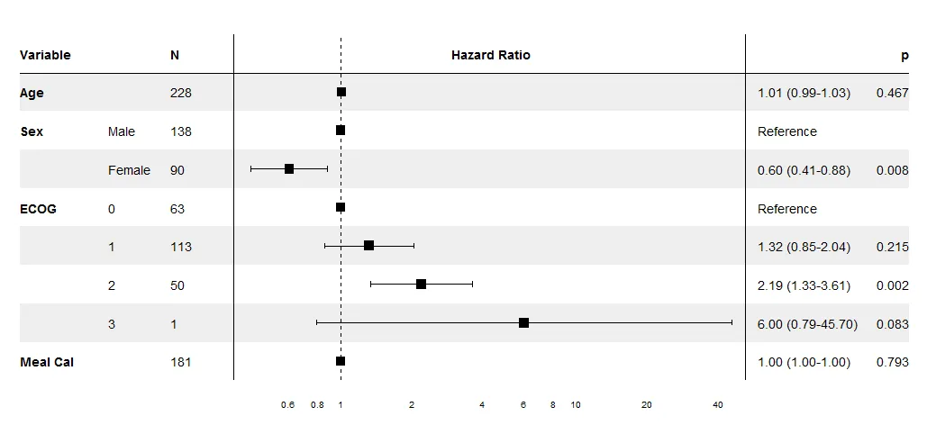
rmeta包的函数forestplot很不错(您可能可以根据需要进行自定义)。虽然它基于grid,而不是ggplot。 - Cath