Python中的反距离加权(IDW)插值

49

问题:

如何在Python中计算逆距离加权(IDW)插值的最佳方法,用于点位置?

背景:

目前我正在使用RPy2与R及其gstat模块进行接口交互。不幸的是,gstat模块与arcgisscripting冲突,我通过在单独的进程中运行基于RPy2的分析来解决了这个问题。即使这个问题在最近/未来的版本中得到解决,并且可以提高效率,我仍然希望不依赖安装R。

gstat网站提供了一个独立的可执行文件,更容易与我的python脚本一起打包,但我仍希望有一个不需要多次写入磁盘和启动外部进程的Python解决方案。我所执行的处理中,对点和值的插值函数的调用次数可以达到20,000次。

我特别需要为点插值,因此使用ArcGIS中的IDW函数生成栅格比使用R还糟糕,就性能而言.....除非有一种有效地屏蔽我所需点的方法。即使进行这种修改,我也不会期望性能表现得很好。我将探索这个选项作为另一种替代方案。更新:这里的问题是你被绑定在你正在使用的单元格大小上。如果你减小单元格大小以获得更好的精度,处理需要很长时间。你还需要通过点提取进行跟进.....总之是一种丑陋的方法,如果你想要特定点的值。

我看过scipy文档,但看起来没有直接计算IDW的简单方法。

我在考虑自己的实现,可能使用一些scipy功能来找到最近的点并计算距离。

我是否遗漏了一些明显的东西?有没有我没见过的Python模块完全符合我的要求?使用scipy辅助创建自己的实现是否明智?

3个回答

44

更新于10月20日:这个类Invdisttree结合了反距离加权和 scipy.spatial.KDTree。 忘记最初的暴力方法; 在我看来,这是散点数据插值的首选方法。

""" invdisttree.py: inverse-distance-weighted interpolation using KDTree
    fast, solid, local
"""
from __future__ import division
import numpy as np
from scipy.spatial import cKDTree as KDTree
    # http://docs.scipy.org/doc/scipy/reference/spatial.html

__date__ = "2010-11-09 Nov"  # weights, doc

#...............................................................................
class Invdisttree:
    """ inverse-distance-weighted interpolation using KDTree:
invdisttree = Invdisttree( X, z )  -- data points, values
interpol = invdisttree( q, nnear=3, eps=0, p=1, weights=None, stat=0 )
    interpolates z from the 3 points nearest each query point q;
    For example, interpol[ a query point q ]
    finds the 3 data points nearest q, at distances d1 d2 d3
    and returns the IDW average of the values z1 z2 z3
        (z1/d1 + z2/d2 + z3/d3)
        / (1/d1 + 1/d2 + 1/d3)
        = .55 z1 + .27 z2 + .18 z3  for distances 1 2 3

    q may be one point, or a batch of points.
    eps: approximate nearest, dist <= (1 + eps) * true nearest
    p: use 1 / distance**p
    weights: optional multipliers for 1 / distance**p, of the same shape as q
    stat: accumulate wsum, wn for average weights

How many nearest neighbors should one take ?
a) start with 8 11 14 .. 28 in 2d 3d 4d .. 10d; see Wendel's formula
b) make 3 runs with nnear= e.g. 6 8 10, and look at the results --
    |interpol 6 - interpol 8| etc., or |f - interpol*| if you have f(q).
    I find that runtimes don't increase much at all with nnear -- ymmv.

p=1, p=2 ?
    p=2 weights nearer points more, farther points less.
    In 2d, the circles around query points have areas ~ distance**2,
    so p=2 is inverse-area weighting. For example,
        (z1/area1 + z2/area2 + z3/area3)
        / (1/area1 + 1/area2 + 1/area3)
        = .74 z1 + .18 z2 + .08 z3  for distances 1 2 3
    Similarly, in 3d, p=3 is inverse-volume weighting.

Scaling:
    if different X coordinates measure different things, Euclidean distance
    can be way off.  For example, if X0 is in the range 0 to 1
    but X1 0 to 1000, the X1 distances will swamp X0;
    rescale the data, i.e. make X0.std() ~= X1.std() .

A nice property of IDW is that it's scale-free around query points:
if I have values z1 z2 z3 from 3 points at distances d1 d2 d3,
the IDW average
    (z1/d1 + z2/d2 + z3/d3)
    / (1/d1 + 1/d2 + 1/d3)
is the same for distances 1 2 3, or 10 20 30 -- only the ratios matter.
In contrast, the commonly-used Gaussian kernel exp( - (distance/h)**2 )
is exceedingly sensitive to distance and to h.

    """
# anykernel( dj / av dj ) is also scale-free
# error analysis, |f(x) - idw(x)| ? todo: regular grid, nnear ndim+1, 2*ndim

    def __init__( self, X, z, leafsize=10, stat=0 ):
        assert len(X) == len(z), "len(X) %d != len(z) %d" % (len(X), len(z))
        self.tree = KDTree( X, leafsize=leafsize )  # build the tree
        self.z = z
        self.stat = stat
        self.wn = 0
        self.wsum = None;

    def __call__( self, q, nnear=6, eps=0, p=1, weights=None ):
            # nnear nearest neighbours of each query point --
        q = np.asarray(q)
        qdim = q.ndim
        if qdim == 1:
            q = np.array([q])
        if self.wsum is None:
            self.wsum = np.zeros(nnear)

        self.distances, self.ix = self.tree.query( q, k=nnear, eps=eps )
        interpol = np.zeros( (len(self.distances),) + np.shape(self.z[0]) )
        jinterpol = 0
        for dist, ix in zip( self.distances, self.ix ):
            if nnear == 1:
                wz = self.z[ix]
            elif dist[0] < 1e-10:
                wz = self.z[ix[0]]
            else:  # weight z s by 1/dist --
                w = 1 / dist**p
                if weights is not None:
                    w *= weights[ix]  # >= 0
                w /= np.sum(w)
                wz = np.dot( w, self.z[ix] )
                if self.stat:
                    self.wn += 1
                    self.wsum += w
            interpol[jinterpol] = wz
            jinterpol += 1
        return interpol if qdim > 1  else interpol[0]

#...............................................................................
if __name__ == "__main__":
    import sys

    N = 10000
    Ndim = 2
    Nask = N  # N Nask 1e5: 24 sec 2d, 27 sec 3d on mac g4 ppc
    Nnear = 8  # 8 2d, 11 3d => 5 % chance one-sided -- Wendel, mathoverflow.com
    leafsize = 10
    eps = .1  # approximate nearest, dist <= (1 + eps) * true nearest
    p = 1  # weights ~ 1 / distance**p
    cycle = .25
    seed = 1

    exec "\n".join( sys.argv[1:] )  # python this.py N= ...
    np.random.seed(seed )
    np.set_printoptions( 3, threshold=100, suppress=True )  # .3f

    print "\nInvdisttree:  N %d  Ndim %d  Nask %d  Nnear %d  leafsize %d  eps %.2g  p %.2g" % (
        N, Ndim, Nask, Nnear, leafsize, eps, p)

    def terrain(x):
        """ ~ rolling hills """
        return np.sin( (2*np.pi / cycle) * np.mean( x, axis=-1 ))

    known = np.random.uniform( size=(N,Ndim) ) ** .5  # 1/(p+1): density x^p
    z = terrain( known )
    ask = np.random.uniform( size=(Nask,Ndim) )

#...............................................................................
    invdisttree = Invdisttree( known, z, leafsize=leafsize, stat=1 )
    interpol = invdisttree( ask, nnear=Nnear, eps=eps, p=p )

    print "average distances to nearest points: %s" % \
        np.mean( invdisttree.distances, axis=0 )
    print "average weights: %s" % (invdisttree.wsum / invdisttree.wn)
        # see Wikipedia Zipf's law
    err = np.abs( terrain(ask) - interpol )
    print "average |terrain() - interpolated|: %.2g" % np.mean(err)

    # print "interpolate a single point: %.2g" % \
    #     invdisttree( known[0], nnear=Nnear, eps=eps )

1
@majgis,不用客气。N=100000 Nask=100000 大约需要 24 秒 2D,27 秒 3D,在我的老 mac G4 PPC 上。(对于将 2D 数据插值到均匀网格上,matplotlib.delaunay 的速度大约是 ~10 倍快的--请参见 http://www.scipy.org/Cookbook/Matplotlib/Gridding_irregularly_spaced_data) - denis
2
请查看此处的警告:https://dev59.com/M2025IYBdhLWcg3wEhhb:“在几乎所有情况下,IDW都是一个可怕的选择...”。尽管如此,对于*您的*数据,IDW可能具有合理的简单性、速度和平滑性的组合。 - denis
@denfromufa,http://creativecommons.org/licenses/by-nc-sa/3.0/ 非商业使用。可以吗? - denis
@denis,那么它就无法集成到scipy中。 - denfromufa
@mfgeng,不知道。你的macOS Python Scipy版本是什么?在更少的点/不同的参数下会崩溃吗? - denis
显示剩余3条评论

42

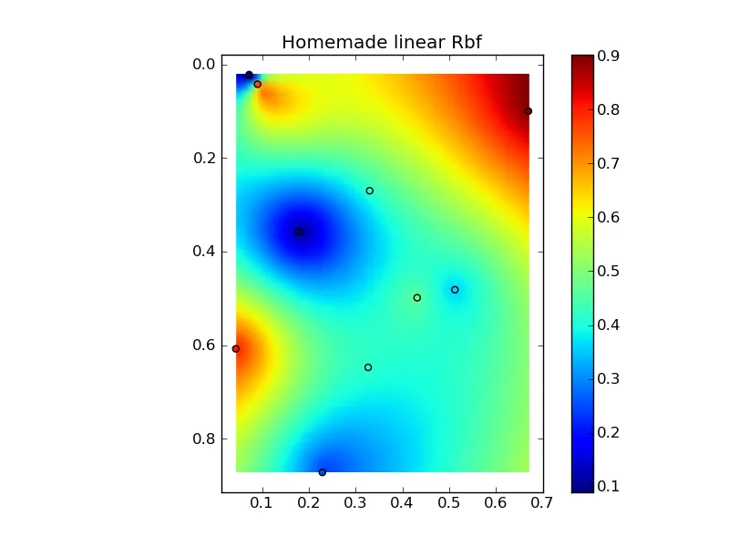
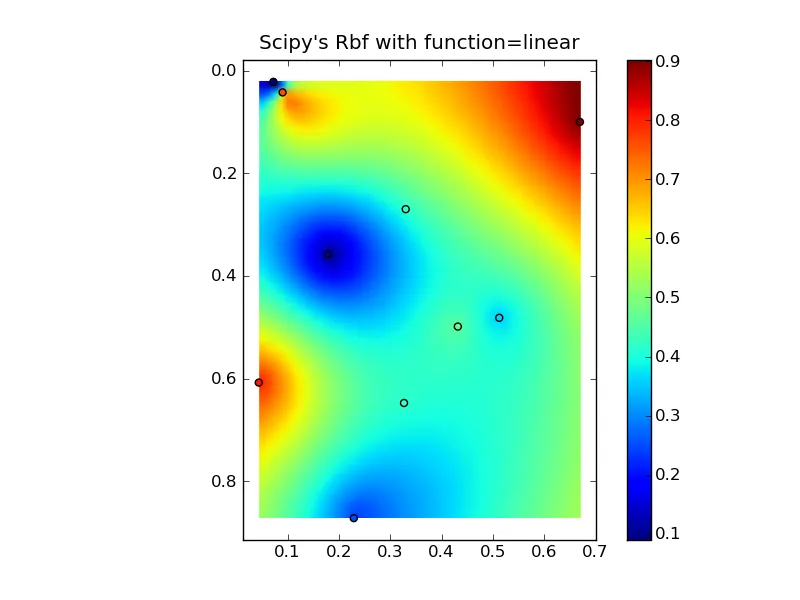
编辑:@Denis 是正确的,一个线性的Rbf(例如 scipy.interpolate.Rbf 并且 "function='linear'") 和 IDW 不同...

(请注意,如果你使用大量点,则所有这些方法都会使用过多的内存!)
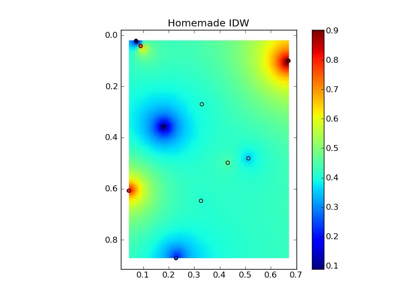
以下是IDW的一个简单示例:

def simple_idw(x, y, z, xi, yi):
    dist = distance_matrix(x,y, xi,yi)

    # In IDW, weights are 1 / distance
    weights = 1.0 / dist

    # Make weights sum to one
    weights /= weights.sum(axis=0)

    # Multiply the weights for each interpolated point by all observed Z-values
    zi = np.dot(weights.T, z)
    return zi

然而,这里是线性Rbf的定义:

def linear_rbf(x, y, z, xi, yi):
    dist = distance_matrix(x,y, xi,yi)

    # Mutual pariwise distances between observations
    internal_dist = distance_matrix(x,y, x,y)

    # Now solve for the weights such that mistfit at the observations is minimized
    weights = np.linalg.solve(internal_dist, z)

    # Multiply the weights for each interpolated point by the distances
    zi =  np.dot(dist.T, weights)
    return zi

(在这里使用distance_matrix函数:)
def distance_matrix(x0, y0, x1, y1):
    obs = np.vstack((x0, y0)).T
    interp = np.vstack((x1, y1)).T

    # Make a distance matrix between pairwise observations
    # Note: from <https://dev59.com/IHI-5IYBdhLWcg3wZ3jC>
    # (Yay for ufuncs!)
    d0 = np.subtract.outer(obs[:,0], interp[:,0])
    d1 = np.subtract.outer(obs[:,1], interp[:,1])

    return np.hypot(d0, d1)

将所有内容组合成一个漂亮的复制粘贴示例,可以得到一些快速比较图: 自制IDW示例图
(来源:www.geology.wisc.edu上的jkington
自制线性RBF示例图
(来源:www.geology.wisc.edu上的jkington
Scipy的线性RBF示例图
(来源:www.geology.wisc.edu上的jkington
import numpy as np
import matplotlib.pyplot as plt
from scipy.interpolate import Rbf

def main():
    # Setup: Generate data...
    n = 10
    nx, ny = 50, 50
    x, y, z = map(np.random.random, [n, n, n])
    xi = np.linspace(x.min(), x.max(), nx)
    yi = np.linspace(y.min(), y.max(), ny)
    xi, yi = np.meshgrid(xi, yi)
    xi, yi = xi.flatten(), yi.flatten()

    # Calculate IDW
    grid1 = simple_idw(x,y,z,xi,yi)
    grid1 = grid1.reshape((ny, nx))

    # Calculate scipy's RBF
    grid2 = scipy_idw(x,y,z,xi,yi)
    grid2 = grid2.reshape((ny, nx))

    grid3 = linear_rbf(x,y,z,xi,yi)
    print grid3.shape
    grid3 = grid3.reshape((ny, nx))


    # Comparisons...
    plot(x,y,z,grid1)
    plt.title('Homemade IDW')

    plot(x,y,z,grid2)
    plt.title("Scipy's Rbf with function=linear")

    plot(x,y,z,grid3)
    plt.title('Homemade linear Rbf')

    plt.show()

def simple_idw(x, y, z, xi, yi):
    dist = distance_matrix(x,y, xi,yi)

    # In IDW, weights are 1 / distance
    weights = 1.0 / dist

    # Make weights sum to one
    weights /= weights.sum(axis=0)

    # Multiply the weights for each interpolated point by all observed Z-values
    zi = np.dot(weights.T, z)
    return zi

def linear_rbf(x, y, z, xi, yi):
    dist = distance_matrix(x,y, xi,yi)

    # Mutual pariwise distances between observations
    internal_dist = distance_matrix(x,y, x,y)

    # Now solve for the weights such that mistfit at the observations is minimized
    weights = np.linalg.solve(internal_dist, z)

    # Multiply the weights for each interpolated point by the distances
    zi =  np.dot(dist.T, weights)
    return zi


def scipy_idw(x, y, z, xi, yi):
    interp = Rbf(x, y, z, function='linear')
    return interp(xi, yi)

def distance_matrix(x0, y0, x1, y1):
    obs = np.vstack((x0, y0)).T
    interp = np.vstack((x1, y1)).T

    # Make a distance matrix between pairwise observations
    # Note: from <https://dev59.com/IHI-5IYBdhLWcg3wZ3jC>
    # (Yay for ufuncs!)
    d0 = np.subtract.outer(obs[:,0], interp[:,0])
    d1 = np.subtract.outer(obs[:,1], interp[:,1])

    return np.hypot(d0, d1)


def plot(x,y,z,grid):
    plt.figure()
    plt.imshow(grid, extent=(x.min(), x.max(), y.max(), y.min()))
    plt.hold(True)
    plt.scatter(x,y,c=z)
    plt.colorbar()

if __name__ == '__main__':
    main()

function="linear" 是 r,而不是 1/r。(这有关系吗?有半打的 function= 选择,它们大相径庭——有些对某些数据效果很好。) - denis
1
@Denis:它使用1/function()来加权。文档在这方面可能需要更清晰,但其他方式都没有意义。否则,距离插值点较远的点将被赋予更高的权重,并且在特定点附近的插值值将具有最接近最远点的值。函数的选择很重要(非常!),IDW通常是错误的选择。然而,目标是产生对进行插值的人看起来合理的结果,因此如果IDW有效,则可以使用它。Scipy的Rbf不会给您太多灵活性。 - Joe Kington
@joe,使用http://en.wikipedia.org/wiki/Radial_basis_function作为符号:phi(r)高斯和反多项式随距离减少,其他随距离增加?! Rbf在cj处精确解决Aw = z(w系数可以变化很多,打印rbf.A rbf.nodes);然后对于phi(r) = r,y(x) = sum(wj |x - cj|),奇怪。稍后会发布(mho of)逆距离加权,然后我们可以进行比较。 - denis
@Denis,谢谢!总有一天我会的,但得等到初试之后。 (研究生有点耗时间!)顺便说一句,我相信是你在一段时间前在scipy邮件列表上就“插值抱怨”问题给我发了电子邮件。很抱歉我从未回复!同样,总有一天我会写一篇博客文章或类似的东西... - Joe Kington
如何获取创建的图像范围以将其作为叠加图层放置在地图上。我尝试过使用点位置的范围,但存在对齐问题。 - Anju
显示剩余4条评论

3
我也需要快速的东西,我从@joerington的解决方案开始尝试,最终使用了numba。
我经常在scipy、numpy和numba之间进行实验,并选择最佳的一个。对于这个问题,我使用了numba,因为额外的tmp内存可以忽略不计,能够提供超高速度。
使用numpy会有速度和内存的权衡。例如,在16GB内存上,如果您想要计算其他50000个点的插值,则无论如何都会耗尽内存或变得非常缓慢。
因此,为了节省内存,我们需要使用for循环,以便进行最小的临时内存分配。但是,在numpy中编写for循环意味着失去可能的向量化。对此,我们有numba。您可以为接受numpy中的for循环的函数添加numba jit,它将在硬件上有效地向量化并在多核上进行额外的并行处理。它将为巨大的数组情况提供更好的加速,并且您可以在不编写cuda的情况下在GPU上运行它。
一个极其简单的片段是计算距离矩阵,在IDW情况下,我们需要逆距离矩阵。但是即使对于除IDW之外的方法,您也可以做类似的事情。
此外,在计算斜边的自定义方法上,我有一些注意事项here
@nb.njit((nb.float64[:, :], nb.float64[:, :]), parallel=True)
def f2(d0, d1):
    print('Numba with parallel')
    res = np.empty((d0.shape[0], d1.shape[0]), dtype=d0.dtype)
    for i in nb.prange(d0.shape[0]):
        for j in range(d1.shape[0]):
            res[i, j] = np.sqrt((d0[i, 0] - d1[j, 0])**2 + (d0[i, 1] - d1[j, 1])**2)
    return res

Also,最近Numba与scikit兼容,所以这是+1。
参考: 为什么np.hypot和np.subtract.outer与vanilla broadcast相比速度非常快?使用Numba加速numpy并行计算距离矩阵 在numpy中自定义dtype用于纬度、经度等更快的距离矩阵/krigging/IDW插值计算

网页内容由stack overflow 提供, 点击上面的
可以查看英文原文,
原文链接