Python环境下不规则网格的曲面图

Question

Python环境下不规则网格的曲面图

4

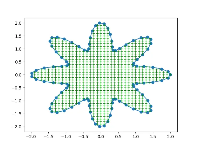
有没有可能为以下区域内的函数创建表面图和等高线图？例如：u(x,y) = x^2 + y^2

该区域由以下方程界定：

r(t) = 1+(cos(4*t))^2, x = r(t)*cos(t),y = r(t)*sin(t), 0 < t < 2*pi

我希望能够得到以下散点图的表面绘制变体。

我还使用了scipy中的griddata，如下所示。

from matplotlib.pyplot  import *
import numpy as np
from mpl_toolkits.mplot3d import Axes3D
from scipy.interpolate import griddata

data = np.array([[ 2.00000000e+00,  0.00000000e+00],
   [ 1.89614525e+00,  1.51126793e-01],
   [ 1.62613327e+00,  2.60869688e-01],
   [ 1.29639187e+00,  3.15328472e-01],
   [ 1.03183519e+00,  3.39805963e-01],
   [ 9.22330309e-01,  3.87424263e-01],
   [ 9.85968247e-01,  5.09806830e-01],
   [ 1.16496791e+00,  7.25092951e-01],
   [ 1.35481653e+00,  1.00089121e+00],
   [ 1.45215333e+00,  1.26290100e+00],
   [ 1.39897768e+00,  1.42707450e+00],
   [ 1.20351374e+00,  1.44074409e+00],
   [ 9.29854857e-01,  1.31248166e+00],
   [ 6.63453200e-01,  1.11474417e+00],
   [ 4.70396020e-01,  9.55864325e-01],
   [ 3.70174853e-01,  9.32786757e-01],
   [ 3.33831717e-01,  1.08590518e+00],
   [ 3.06157327e-01,  1.37738581e+00],
   [ 2.38732323e-01,  1.70413196e+00],
   [ 1.15900227e-01,  1.94068353e+00],
   [-3.96388724e-02,  1.99329358e+00],
   [-1.83621616e-01,  1.84088591e+00],
   [-2.79344160e-01,  1.54430632e+00],
   [-3.22477316e-01,  1.21965478e+00],
   [-3.47231849e-01,  9.87829012e-01],
   [-4.09520279e-01,  9.23088740e-01],
   [-5.55288737e-01,  1.02352335e+00],
   [-7.90735832e-01,  1.21586141e+00],
   [-1.07111976e+00,  1.39113164e+00],
   [-1.31601256e+00,  1.45381050e+00],
   [-1.44544698e+00,  1.36169834e+00],
   [-1.42013085e+00,  1.13913085e+00],
   [-1.26561597e+00,  8.59376173e-01],
   [-1.06700598e+00,  6.06642746e-01],
   [-9.34540362e-01,  4.37040778e-01],
   [-9.54661396e-01,  3.57053472e-01],
   [-1.14896223e+00,  3.28361061e-01],
   [-1.46070082e+00,  2.94327457e-01],
   [-1.77632959e+00,  2.12929020e-01],
   [-1.97334870e+00,  7.85155418e-02],
   [-1.97334870e+00, -7.85155418e-02],
   [-1.77632959e+00, -2.12929020e-01],
   [-1.46070082e+00, -2.94327457e-01],
   [-1.14896223e+00, -3.28361061e-01],
   [-9.54661396e-01, -3.57053472e-01],
   [-9.34540362e-01, -4.37040778e-01],
   [-1.06700598e+00, -6.06642746e-01],
   [-1.26561597e+00, -8.59376173e-01],
   [-1.42013085e+00, -1.13913085e+00],
   [-1.44544698e+00, -1.36169834e+00],
   [-1.31601256e+00, -1.45381050e+00],
   [-1.07111976e+00, -1.39113164e+00],
   [-7.90735832e-01, -1.21586141e+00],
   [-5.55288737e-01, -1.02352335e+00],
   [-4.09520279e-01, -9.23088740e-01],
   [-3.47231849e-01, -9.87829012e-01],
   [-3.22477316e-01, -1.21965478e+00],
   [-2.79344160e-01, -1.54430632e+00],
   [-1.83621616e-01, -1.84088591e+00],
   [-3.96388724e-02, -1.99329358e+00],
   [ 1.15900227e-01, -1.94068353e+00],
   [ 2.38732323e-01, -1.70413196e+00],
   [ 3.06157327e-01, -1.37738581e+00],
   [ 3.33831717e-01, -1.08590518e+00],
   [ 3.70174853e-01, -9.32786757e-01],
   [ 4.70396020e-01, -9.55864325e-01],
   [ 6.63453200e-01, -1.11474417e+00],
   [ 9.29854857e-01, -1.31248166e+00],
   [ 1.20351374e+00, -1.44074409e+00],
   [ 1.39897768e+00, -1.42707450e+00],
   [ 1.45215333e+00, -1.26290100e+00],
   [ 1.35481653e+00, -1.00089121e+00],
   [ 1.16496791e+00, -7.25092951e-01],
   [ 9.85968247e-01, -5.09806830e-01],
   [ 9.22330309e-01, -3.87424263e-01],
   [ 1.03183519e+00, -3.39805963e-01],
   [ 1.29639187e+00, -3.15328472e-01],
   [ 1.62613327e+00, -2.60869688e-01],
   [ 1.89614525e+00, -1.51126793e-01],
   [ 2.00000000e+00, -4.89858720e-16],
   [ 0.00000000e+00, -1.50000000e+00],
   [-1.00000000e+00, -1.00000000e+00],
   [ 0.00000000e+00, -1.00000000e+00],
   [ 1.00000000e+00, -1.00000000e+00],
   [-5.00000000e-01, -5.00000000e-01],
   [ 0.00000000e+00, -5.00000000e-01],
   [ 5.00000000e-01, -5.00000000e-01],
   [-1.50000000e+00,  0.00000000e+00],
   [-1.00000000e+00,  0.00000000e+00],
   [-5.00000000e-01,  0.00000000e+00],
   [ 0.00000000e+00,  0.00000000e+00],
   [ 5.00000000e-01,  0.00000000e+00],
   [ 1.00000000e+00,  0.00000000e+00],
   [ 1.50000000e+00,  0.00000000e+00],
   [ 2.00000000e+00,  0.00000000e+00],
   [-5.00000000e-01,  5.00000000e-01],
   [ 0.00000000e+00,  5.00000000e-01],
   [ 5.00000000e-01,  5.00000000e-01],
   [-1.00000000e+00,  1.00000000e+00],
   [ 0.00000000e+00,  1.00000000e+00],
   [ 1.00000000e+00,  1.00000000e+00],
   [ 0.00000000e+00,  1.50000000e+00]])   
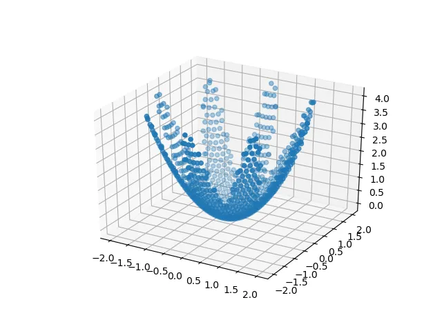
ua = data[:,0]**2+data[:,1]**2 # u=x^2+y^2


xx,yy = np.meshgrid(np.linspace(-2,2,100),np.linspace(-2,2,100))
Ua = griddata((data[:,0],data[:,1]),ua,(xx,yy),method='cubic') 

fig = figure(1)
plot (data[:,0], data[:,1], '*'); # 
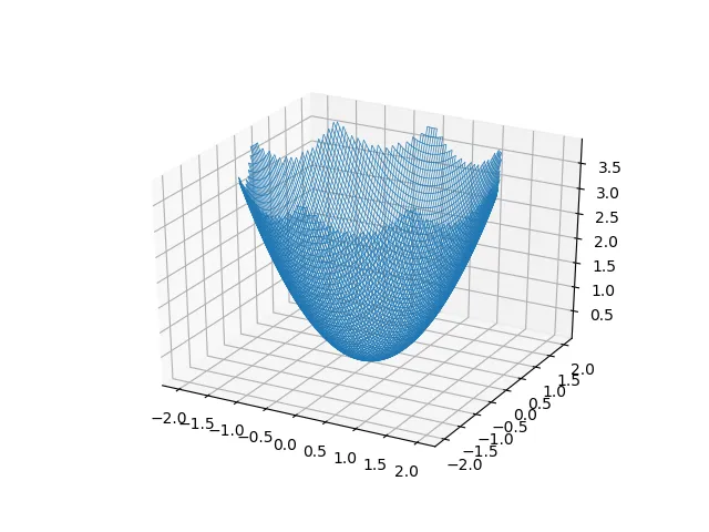
fig = figure(2)
ax = fig.gca(projection='3d')

ax.plot_wireframe(xx,yy,Ua,rstride=1,cstride=1,linewidth=.5)

但结果不如下面这样好：

- user1772257

你用什么代码创建了第二个图？你想让它看起来像什么？ - Joooeey

@Joooeey：我已经添加了代码。正如我所说，我希望得到给定域的曲面图和等高线图。 - user1772257

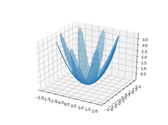
好的。结果有什么问题吗？它显示了正确的域名吗？看起来域名可能不正确。另外，如果您提供一个最小、完整、可验证的示例（MCVE），我可以将其复制到我的IDE中，这将使弄清楚出了什么问题变得更加容易。也就是说，哪里有定义data的代码？ - Joooeey

你展示的是一个表面图。你可以使用 contour(xx, yy, Ua) 得到等高线图。 - Joooeey

我知道这是一个曲面图，但它并不正确。请看散点图。 - user1772257

好的，那么表面图没有像我说的那样在正确的域上绘制。我找到了原因：scipy.interpolate.griddata 在凸包内插值。所以它也在你的叶片之间进行插值。也许你需要一个不同的方法来使它工作。我会看看能否找到任何东西。 - Joooeey

1个回答

网页内容由stack overflow 提供, 点击上面的

可以查看英文原文，
原文链接

- Joooeey · Accepted Answer

首先，在矩形网格上计算函数！

scipy.interpolate.griddata 插值在凸包上。你可以在文档中阅读到这一点。这意味着它还会在你的波峰之间插值。这就是为什么你没有得到正确的定义域。插值本质上也比在网格上直接计算函数不精确。

plot_wireframe 需要一个你已经创建的矩形网格。你只需要在矩形网格上计算函数值即可。如果要仅绘制定义域边界上的值，请将其外部的所有值设置为 np.NaN（非数字）。

以下是实现方法：

import matplotlib.pyplot as plt
import numpy as np

# cartesian coordinates
xx,yy = np.meshgrid(np.linspace(-2,2,100),np.linspace(-2,2,100))

# function value across square domain
Ua = xx**2 + yy**2

# polar coordinates
tt = np.arctan2(yy, xx)
rr = np.sqrt(Ua) # re-using x^2 + y^2 -- only works for this function

# r coordinate of domain boundary
domain_boundary = 1 + (np.cos(4*tt))**2

# function value across actual domain, with rest set to NaN
Ua[rr > domain_boundary] = np.NaN

# plotting
fig = plt.figure(2)
ax = fig.gca(projection='3d')
ax.plot_wireframe(xx,yy,Ua,rstride=1,cstride=1,linewidth=.5)

那个解决方案并不完美，因为你可以在结果中看到矩形网格。你可以尝试使用极坐标来工作，就像这个官方的matplotlib示例中所示的那样。