我有一个关于Wolfram Mathematica的问题。有人知道如何在y轴上绘制图形吗?
希望这个图片能帮助你。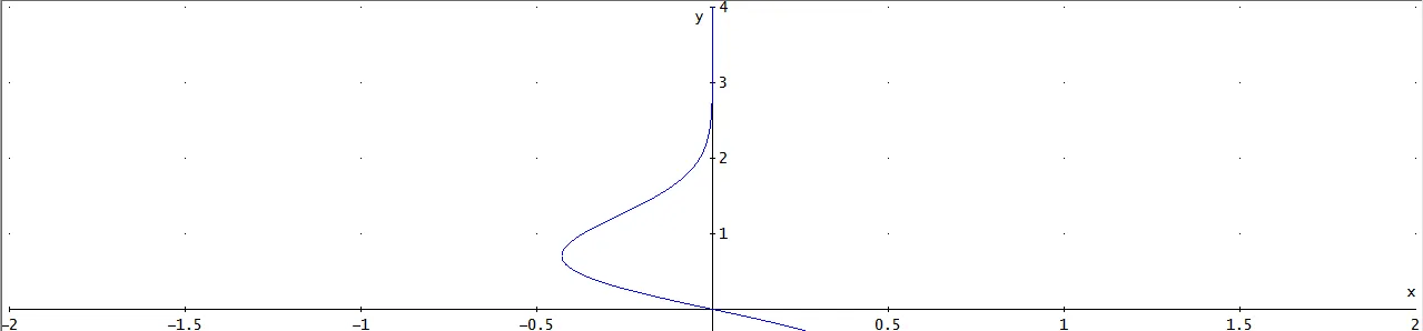
希望这个图片能帮助你。
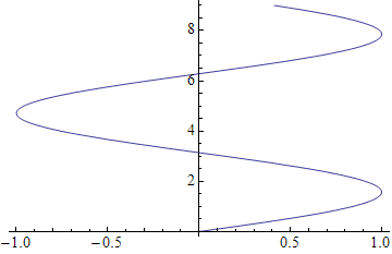
ParametricPlot[{5 Sin[y], y}, {y, -2 \[Pi], 2 \[Pi]},
                Frame -> True,  AxesLabel -> {"x", "y"}]
编辑
到目前为止,所有给出的答案都无法与 Plot 的 Filling 选项一起使用。在这种情况下,Plot 的输出包含一个 GraphicsComplex(顺便说一句,这破坏了 Mr.Wizard 的替换)。要获得填充功能(在没有填充的标准绘图中不起作用),您可以使用以下内容:
Plot[Sin[x], {x, 0, 2 \[Pi]}, Filling -> Axis] /. List[x_, y_] -> List[y, x]
Plot[{Sin[x], .5 Sin[2 x]}, {x, 0, 2 \[Pi]}, Filling -> {1 -> {2}}]
   /. List[x_, y_] -> List[y, x]
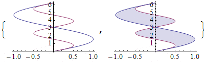
Reverse翻转轴:g = Plot[Sin[x], {x, 0, 9}];
Show[g /. x_Line :> Reverse[x, 3], PlotRange -> Automatic]
只需进行微小的更改,即可适用于使用Filling的图表:
g1 = Plot[{Sin[x], .5 Sin[2 x]}, {x, 0, 2 \[Pi]}];
g2 = Plot[{Sin[x], .5 Sin[2 x]}, {x, 0, 2 \[Pi]}, Filling -> {1 -> {2}}];

Show[# /. x_Line | x_GraphicsComplex :> x~Reverse~3,
     PlotRange -> Automatic] & /@ {g1, g2}
(将:>的右侧替换为MapAt[#~Reverse~2 &, x, 1]可能更加健壮。)
这是我建议使用的形式。 它包括翻转原始PlotRange而不是强制使用PlotRange -> All:
axisFlip = # /. {
   x_Line | x_GraphicsComplex :>
      MapAt[#~Reverse~2 &, x, 1],
   x : (PlotRange -> _) :>
      x~Reverse~2 } &;
用法示例:axisFlip @ g1或axisFlip @ {g1, g2}
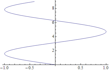
Rotate可以产生不同的效果:
Show[g /. x_Line :> Rotate[x, Pi/2, {0,0}], PlotRange -> Automatic]
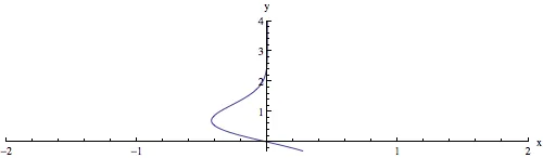
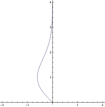
有一种可能性是使用 ParametricPlot,像这样:
ParametricPlot[
  {-y*Exp[-y^2], y}, {y, -0.3, 4},
  PlotRange -> {{-2, 2}, All},
  AxesLabel -> {"x", "y"},
  AspectRatio -> 1/4
]
仅供娱乐:
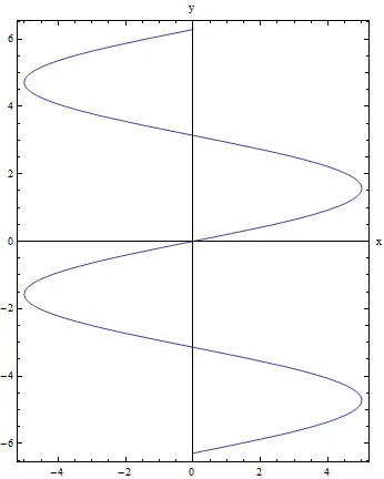
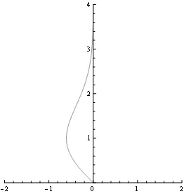
ContourPlot 是另一种选择。使用Thies函数:
ContourPlot[-y*Exp[-y^2/2] - x == 0,
            {x, -2, 2}, {y, 0, 4},
            Axes -> True, Frame -> None]
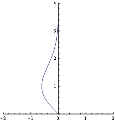
RegionPlot is another
RegionPlot[-y*Exp[-y^2/2] > x,
           {x, -2.1, 2.1}, {y, -.1, 4.1},
           Axes -> True, Frame -> None, PlotStyle -> White,
           PlotRange -> {{-2, 2}, {0, 4}}]
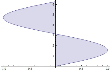
最后,使用ListCurvePathPlot和Solve的方法非常复杂:
Off[Solve::ifun, FindMaxValue::fmgz];

ListCurvePathPlot[
 Join @@
  Table[
        {x, y} /. Solve[-y*Exp[-y^2/2] == x, y],
   {x, FindMaxValue[-y*Exp[-y^2/2], y], 0, .01}],
 PlotRange -> {{-2, 2}, {0, 4}}]

On[Solve::ifun, FindMaxValue::fmgz];
不相关话题
回答Sjoerd的迄今为止给出的答案都不能与Plot的Filling选项一起使用。
回复:不必要。
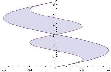
f={.5 Sin[2 y],Sin[y]};
RegionPlot[Min@f<=x<=Max@f,{x,-1,1},{y,-0.1,2.1 Pi},
  Axes->True,Frame->None,
  PlotRange->{{-2,2},{0,2 Pi}},
  PlotPoints->500]
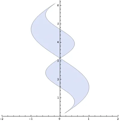
RegionPlot,但它的语法与Plot不同且更加复杂。能够简单地添加Filling -> True更为熟悉。 - Mr.WizardAxesStyle -> Thickness[.1] 进行探索,并取得了非常好的效果。 - Dr. belisarius根据您对轴标签的要求,您可以将原始绘图代码包装在旋转函数中。