我已经在ggplot中使用了两个变量创建了一个图形,并使用facet_grid进行了分面。
我希望每个分面的标题只重复一次,并且位于分面的中央。
例如,在第一行(上部分面)中的零和一将仅出现一次,并位于正中间。
在我的原始图中,每个分面的绘图数量不相等。因此,使用patchwork / cowplot / ggpubr将两个图表拼接在一起并不很好。
我更喜欢仅使用ggplot的解决方案/技巧。
示例数据:
df <- head(mtcars, 5)
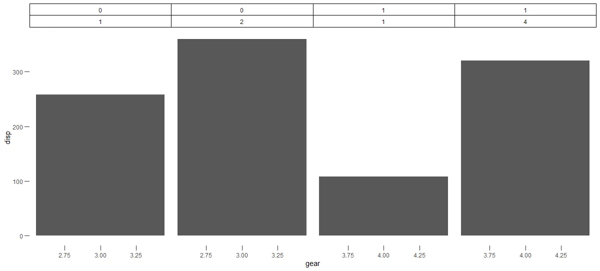
示例图:
df %>%
  ggplot(aes(gear, disp)) +
  geom_bar(stat = "identity") +
  facet_grid(~am + carb,
             space = "free_x",
             scales = "free_x") +
  ggplot2::theme(
    panel.spacing.x = unit(0,"cm"),
    axis.ticks.length=unit(.25, "cm"),
    strip.placement = "outside",
    legend.position = "top",
    legend.justification = "center",
    legend.direction = "horizontal",
    legend.key.size = ggplot2::unit(1.5, "lines"),
    # switch off the rectangle around symbols
    legend.key = ggplot2::element_blank(),
    legend.key.width = grid::unit(2, "lines"),
    # # facet titles
    strip.background = ggplot2::element_rect(
      colour = "black",
      fill = "white"),
    panel.background = ggplot2::element_rect(
      colour = "white",
      fill = "white"),
    panel.grid.major = element_blank(),
    panel.grid.minor = element_blank())
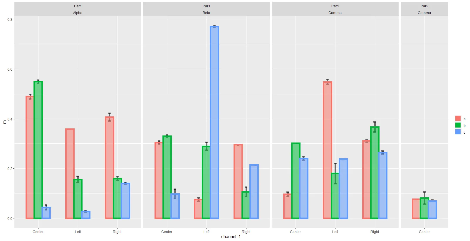
编辑 - 新数据
我创建了一个样本数据,更准确地类似于我的实际数据。
structure(list(par = c("Par1", "Par1", "Par1", "Par1", "Par1",
"Par1", "Par1", "Par1", "Par1", "Par1", "Par1", "Par1", "Par1",
"Par1", "Par1", "Par1", "Par1", "Par1", "Par1", "Par1", "Par1",
"Par1", "Par1", "Par1", "Par1", "Par1", "Par1", "Par2", "Par2",
"Par2"), channel_1 = structure(c(1L, 1L, 1L, 1L, 1L, 1L, 1L,
1L, 1L, 6L, 6L, 6L, 6L, 6L, 6L, 6L, 6L, 6L, 11L, 11L, 11L, 11L,
11L, 11L, 11L, 11L, 11L, 1L, 1L, 1L), .Label = c("Center", "Left \nFrontal",
"Left \nFrontal Central", "Left \nCentral Parietal", "Left \nParietal Ooccipital",
"Left", "Right \nFrontal", "Right \nFrontal Central", "Right \nCentral Parietal",
"Right \nParietal Ooccipital", "Right"), class = "factor"), freq = structure(c(1L,
1L, 1L, 2L, 2L, 2L, 3L, 3L, 3L, 1L, 1L, 1L, 2L, 2L, 2L, 3L, 3L,
3L, 1L, 1L, 1L, 2L, 2L, 2L, 3L, 3L, 3L, 3L, 3L, 3L), .Label = c("Alpha",
"Beta", "Gamma"), class = "factor"), group = c("a", "b", "c",
"a", "b", "c", "a", "b", "c", "a", "b", "c", "a", "b", "c", "a",
"b", "c", "a", "b", "c", "a", "b", "c", "a", "b", "c", "a", "b",
"c"), m = c(0.488630500442935, 0.548666228768508, 0.0441536349332613,
0.304475866391531, 0.330039488441422, 0.0980622573307064, 0.0963996979198171,
0.301679466108907, 0.240618782227119, 0.35779695722622, 0.156116647839907,
0.0274546218676152, 0.0752501569920047, 0.289342864254614, 0.770518960576786,
0.548130676907356, 0.180158614358946, 0.238520826021687, 0.406326198917495,
0.159739769132509, 0.140739952534666, 0.295427640977557, 0.106130817023844,
0.214006898241167, 0.31081727835652, 0.366982521446529, 0.264432086988446,
0.0761271112139142, 0.0811642772125171, 0.0700455890939194),
    se = c(0.00919040825504951, 0.00664655073810519, 0.0095517721611042,
    0.00657090455386036, 0.00451135146762504, 0.0188625074573698,
    0.00875378313351897, 0.000569521129673224, 0.00691447732630984,
    0.000241814142091401, 0.0124584589176995, 0.00366855139256551,
    0.0072981677277562, 0.0160663614099261, 0.00359337442316408,
    0.00919725279757502, 0.040856967817406, 0.00240910563984416,
    0.0152236046767608, 0.00765487375180611, 0.00354140237391633,
    0.00145468584619171, 0.0185141245423404, 0.000833307847848054,
    0.0038193622895167, 0.0206130436440409, 0.0066911922721337,
    7.3079999953491e-05, 0.0246233416039572, 0.00328150956514463
    )), row.names = c(NA, -30L), class = c("tbl_df", "tbl", "data.frame"
))
剧情:
df %>%
  ggplot(aes(channel_1, m,
             group = group,
             fill = group,
             color = group)) +
  facet_grid(~par + freq,
             space="free_x",
             scales="free_x") +
  geom_errorbar(
    aes(min = m - se, ymax = m + se, alpha = 0.01),
    width = 0.2, size = 2, color = "black",
    position = position_dodge(width = 0.6)) +
  geom_bar(stat = "identity",
           position = position_dodge(width = 0.6),
           # color = "black",
           # fill = "white",
           width = 0.6,
           size = 2, aes(alpha = 0.01))  +
  scale_shape_manual(values = c(1, 8, 5)) +
  labs(
    color = "",
    fill = "",
    shape = "") +
  guides(
    color = FALSE,
    shape = FALSE) +
  scale_alpha(guide = "none")