在Python中将2D数据重新网格化到给定坐标的较大2D网格上

Question

我有一个二维数组data，我希望将其添加到更大的二维数组frame中，添加位置是一些给定的非整数坐标coords。这个想法是在新坐标处将data插值到frame上，使其居中。

一些玩具数据：

# A gaussian to add to the frame
x, y = np.meshgrid(np.linspace(-1,1,10), np.linspace(-1,1,10))
data = 50*np.exp(-np.sqrt(x**2+y**2)**2)

# The frame to add the gaussian to
frame = np.random.normal(size=(100,50))

# The desired (x,y) location of the gaussian center on the new frame
coords = 23.4, 22.6

这是我的想法。我想把这个：

添加到这个中：

以得到这个结果：

如果坐标是整数(索引)，当然可以像这样简单地将它们相加：

frame[23:33,22:32] += data

但我希望能够指定非整数坐标，以便对 data 进行重新网格化并添加到 frame 中。

我已经研究了 PIL.Image 方法，但我的用例仅针对二维数据，不是图片。有没有办法只使用 scipy 来完成此操作？是否可以使用 interp2d 或类似的函数来实现？任何指导将不胜感激！

- Joe Flip

---

frame 的坐标是什么？所以你只想用 data 替换 frame 的一部分？ - anishtain4

@anishtain4 噢，抱歉。frame的坐标只是索引，而不是替换。我想要添加它。 - Joe Flip

那么你想调整数据大小吗？如果索引与frame完全重叠，那么我的答案是最简单的方法，因为shift可以完成。如果不是，则另一个答案是最通用和最好的。 - Chiel

data图像中的像素“坐标”（x和y）间隔为0.222(2)个单位（“像素比例尺”）-请参见np.linspace(-1,1,10)，因此，如果映射到输出frame网格上（假设间距为1个像素），则将导致data图像在放置到输出frame图像中时缩小至仅2个像素大小。 但是，您的示例图像没有显示这种缩放变换。因此，我的问题是：linspace用于生成“真实”的坐标网格还是仅用于为高斯和data像素的像素网格创建网格？ - AGN Gazer

你有机会尝试我的答案吗？我相信它也可以以更简单的方式给你相同的结果。 - anishtain4

Answer 1

Scipy的scipy.ndimage.interpolation中的shift函数是您要寻找的，只要data和frame之间的网格间距重叠。如果不是，可以看看其他答案。shift函数可以接受浮点数作为输入，并进行样条插值。首先，将数据放入与帧一样大的数组中，然后进行移位，最后加上它。请确保颠倒坐标列表，因为x是numpy数组中最右边的维度之一。shift的一个好处是它将超出边界的值设置为零。

import numpy as np
import matplotlib.pyplot as plt
from scipy.ndimage.interpolation import shift

# A gaussian to add to the frame.
x, y = np.meshgrid(np.linspace(-1,1,10), np.linspace(-1,1,10))
data = 50*np.exp(-np.sqrt(x**2+y**2)**2)

# The frame to add the gaussian to
frame = np.random.normal(size=(100,50))
x_frame = np.arange(50)
y_frame = np.arange(100)

# The desired (x,y) location of the gaussian center on the new frame.
coords = np.array([23.4, 22.6])

# First, create a frame as large as the frame.
data_large = np.zeros(frame.shape)
data_large[:data.shape[0], :data.shape[1]] = data[:,:]

# Subtract half the distance as the bottom left is at 0,0 instead of the center.
# The shift of 4.5 is because data is 10 points wide.
# Reverse the coords array as x is the last coordinate.
coords_shift = -4.5
data_large = shift(data_large, coords[::-1] + coords_shift)

frame += data_large

# Plot the result and add lines to indicate to coordinates
plt.figure()
plt.pcolormesh(x_frame, y_frame, frame, cmap=plt.cm.jet)
plt.axhline(coords[1], color='w')
plt.axvline(coords[0], color='w')
plt.colorbar()
plt.gca().invert_yaxis()
plt.show()

该脚本给出了以下图形，其中所需的坐标用白色虚线标示。

- Chiel

---

请查看我对答案的最新编辑。我没有发现你的答案有任何问题，我认为你应该保留它：在我看来，它比我的略微简单（但不是很多）。在我看来，这是一个有效的答案，你应该保留它。 - AGN Gazer

另外，我认为你的 coords_shift=-5 应该是 -4.5，因为高斯函数的中心在 4.5 个像素处。这不是一个大问题，实际上它取决于采用哪种约定：原点在角落还是在像素的中心。(我不得不将 coords_shift 设置为 -4.5 才能与我的输出进行比较。) - AGN Gazer

太好了，您已经恢复了您的答案！如果没有更多选项，那就太可惜了。 - AGN Gazer

Answer 2

一种可能的解决方案是使用scipy.interpolate.RectBivariateSpline。在下面的代码中，x_0和y_0是数据中特征的坐标（即您示例中高斯分布的中心位置）需要映射到由coords给出的坐标。这种方法有几个优点：

1. 如果您需要将相同的对象“放置”到输出frame中的多个位置，则只需计算样条曲线一次（但要评估多次）。

2. 如果您实际上需要计算模型在像素上的积分通量，则可以使用scipy.interpolate.RectBivariateSpline的integral method。

使用样条插值重新采样：

from scipy.interpolate import RectBivariateSpline
x = np.arange(data.shape[1], dtype=np.float)
y = np.arange(data.shape[0], dtype=np.float)
kx = 3; ky = 3; # spline degree
spline = RectBivariateSpline(
    x, y, data.T, kx=kx, ky=ky, s=0
)

# Define coordinates of a feature in the data array.
# This can be the center of the Gaussian:
x_0 = (data.shape[1] - 1.0) / 2.0
y_0 = (data.shape[0] - 1.0) / 2.0

# create output grid, shifted as necessary:
yg, xg = np.indices(frame.shape, dtype=np.float64)
xg += x_0 - coords[0] # see below how to account for pixel scale change
yg += y_0 - coords[1] # see below how to account for pixel scale change

# resample and fill extrapolated points with 0:
resampled_data = spline.ev(xg, yg)
extrapol = (((xg < -0.5) | (xg >= data.shape[1] - 0.5)) |
            ((yg < -0.5) | (yg >= data.shape[0] - 0.5)))
resampled_data[extrapol] = 0

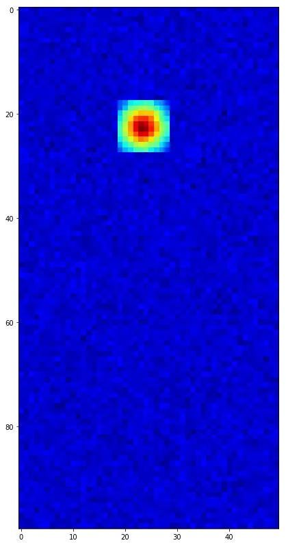
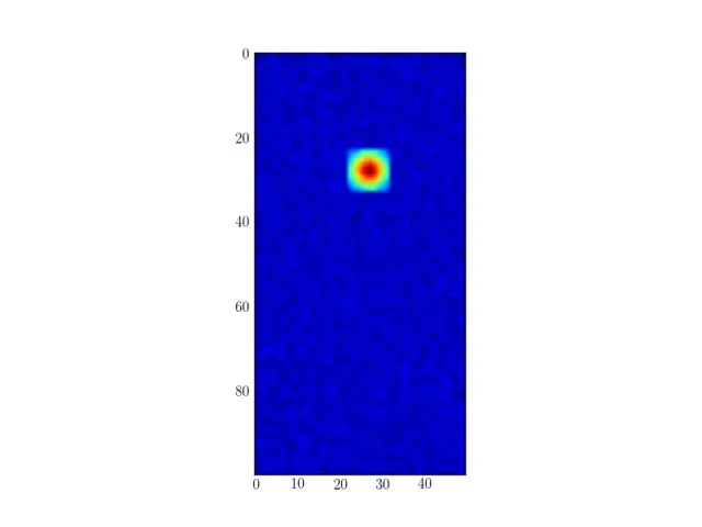
现在绘制frame和重采样的data:

plt.figure(figsize=(14, 14));
plt.imshow(frame+resampled_data, cmap=plt.cm.jet,
          origin='upper', interpolation='none', aspect='equal')
plt.show()

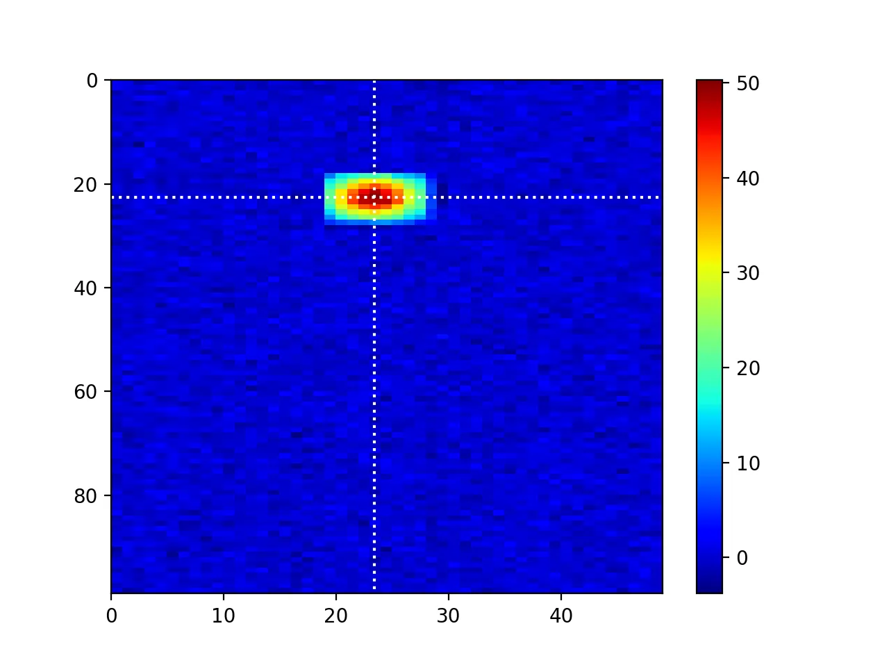
如果你也希望允许比例变化，那么请将上面计算xg和yg的代码用以下代码替换:

coords = 20, 80 # change coords to easily identifiable (in plot) values
zoom_x = 2 # example scale change along X axis
zoom_y = 3 # example scale change along Y axis
yg, xg = np.indices(frame.shape, dtype=np.float64)
xg = (xg - coords[0]) / zoom_x + x_0
yg = (yg - coords[1]) / zoom_y + y_0

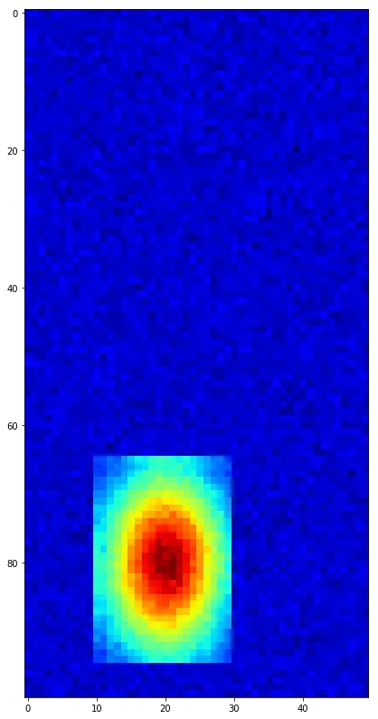
根据您的示例，最有可能这正是您实际想要的。具体而言，data中像素的坐标以0.222（2）距离单位“间隔”。因此，对于您特定的示例（无论是意外还是故意），您实际上具有0.222（2）的缩放因子。在这种情况下，您的data图像将在输出帧中缩小到几乎2个像素。

---

与@Chiel答案的比较

在下面的图像中，我比较了我的方法（左侧）、@Chiel的方法（中间）和差异（右侧面板）的结果：

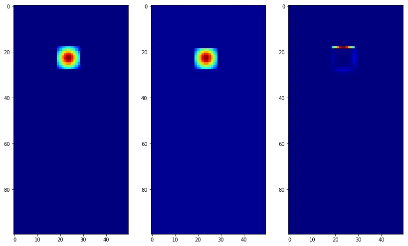
基本上，这两种方法非常相似，甚至可能使用相同的算法（我没有查看shift的代码，但根据描述 - 它也使用样条曲线）。从比较图像中可以看出，最大的差异在于边缘，并且由于我不知道原因，shift似乎会过早地截断移动后的图像。

我认为最大的区别在于我的方法允许像素比例的更改，它还允许重复使用相同的插值器将原始图像放置在输出帧的不同位置。 @Chiel的方法有点简单，但（我不喜欢的是）它需要创建一个更大的数组（data_large），将原始图像放置在角落里。

- AGN Gazer

---

@Chiel 你确定吗？虽然我还没有测试你的答案，但是目前为止似乎没有什么问题。 你能否请恢复一下它，至少暂时这样，我可以测试一下？ - AGN Gazer

我恢复了我的答案。我添加了它可以工作的条件，以及何时需要使用你的解决方案。你的解决方案更通用，但如果shift足够的话，它是首选。 - Chiel

很好，你比较了答案。 - Chiel

Answer 3

虽然其他答案已经详细解释了，但这是我的懒惰解决方案：

xc,yc = 23.4, 22.6
x, y = np.meshgrid(np.linspace(-1,1,10)-xc%1, np.linspace(-1,1,10)-yc%1)
data = 50*np.exp(-np.sqrt(x**2+y**2)**2)
frame = np.random.normal(size=(100,50))
frame[23:33,22:32] += data

这就是你喜欢的方式。正如你所提到的，两者的坐标是相同的，因此data的原点在索引之间的某个位置。现在只需在第二行中将其简单地移动到离网格点（余数为1）所需的距离即可（你可能需要翻转符号，但我认为这是正确的）。

- anishtain4