如何在同一面板中绘制不同GAM的平滑组件？

Question

我有两个广义相加模型（GAM），它们具有相同的预测变量，但具有不同的自变量。我想将这两个GAM组合成一组图，其中每个预测变量的平滑部分（偏残差）位于同一个面板中（可以用颜色区分）。可重复的示例：

# Required packages
require(mgcv)
require(mgcViz)

# Dataset
data("swiss")

# GAM models
fit1 <- mgcv::gam(Fertility ~ s(Examination) + s(Education), data = swiss)
fit2 <- mgcv::gam(Agriculture ~ s(Examination) + s(Education), data = swiss)

# Converting GAM objects to a gamViz objects
viz_fit1 <- mgcViz::getViz(fit1)
viz_fit2 <- mgcViz::getViz(fit2)

# Make plotGAM objects
trt_fit1 <- plot(viz_fit1, allTerms = T) + l_fitLine()
trt_fit2 <- plot(viz_fit2, allTerms = T) + l_fitLine()

# Print plots
print(trt_fit1, pages = 1)
print(trt_fit2, pages = 1)

fit1的图像如下：

而fit2的图像则是这样的：

因此，我希望将两个检查合并为一个面板，并将两个教育合并为另一个面板，以不同的颜色/线型显示来自不同GAM的自变量。

- tolonen

---

但是你的两个结果变量不会有不同的y轴刻度吗？你想要一个次要轴吗？还是这两个结果可以用相同的刻度表示？ - Allan Cameron

它们将具有不同的y轴刻度，这是正确的。然而，它们具有非常相似的范围，因此仍然可以使用相同的y轴轻松解释它们。 - tolonen

Answer 1

你可以使用我的{gratia}和compare_smooths()函数来完成这个操作：

library("gratia")
library("mgcv")

# Dataset 
data("swiss") 

# GAM models 
fit1 <- gam(Fertility ~ s(Examination) + s(Education),
            data = swiss, method = "REML")
fit2 <- gam(Agriculture ~ s(Examination) + s(Education),
            data = swiss, method = "REML")

# create and object that contains the info to compare smooths
comp <- compare_smooths(fit1, fit2)

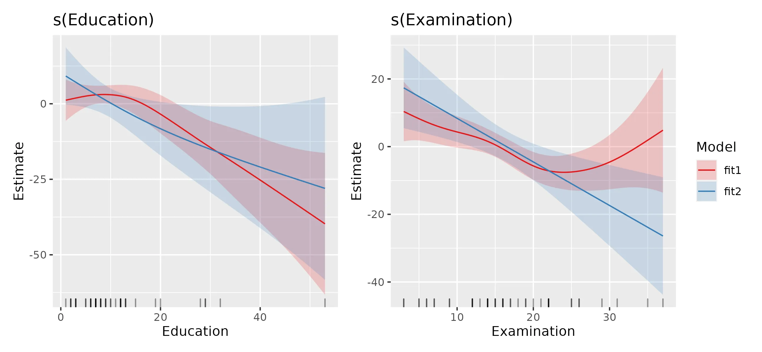
# plot
draw(comp)

这会产生

compare_smooth()的输出是一个嵌套数据框（tibble）。

r$> comp                                                                        
# A tibble: 4 × 5
  model smooth         type  by    data              
  <chr> <chr>          <chr> <chr> <list>            
1 fit1  s(Education)   TPRS  NA    <tibble [100 × 3]>
2 fit2  s(Education)   TPRS  NA    <tibble [100 × 3]>
3 fit1  s(Examination) TPRS  NA    <tibble [100 × 3]>
4 fit2  s(Examination) TPRS  NA    <tibble [100 × 3]>

因此，如果您想自定义绘图等内容，您需要知道如何使用嵌套数据框架或只需执行

library("tidyr")
unnest(comp, data)

这将使您得到：

r$> unnest(comp, data)                                                          
# A tibble: 400 × 8
   model smooth       type  by      est    se Education Examination
   <chr> <chr>        <chr> <chr> <dbl> <dbl>     <dbl>       <dbl>
 1 fit1  s(Education) TPRS  NA     1.19  3.48      1             NA
 2 fit1  s(Education) TPRS  NA     1.37  3.20      1.53          NA
 3 fit1  s(Education) TPRS  NA     1.56  2.94      2.05          NA
 4 fit1  s(Education) TPRS  NA     1.75  2.70      2.58          NA
 5 fit1  s(Education) TPRS  NA     1.93  2.49      3.10          NA
 6 fit1  s(Education) TPRS  NA     2.11  2.29      3.63          NA
 7 fit1  s(Education) TPRS  NA     2.28  2.11      4.15          NA
 8 fit1  s(Education) TPRS  NA     2.44  1.95      4.68          NA
 9 fit1  s(Education) TPRS  NA     2.59  1.82      5.20          NA
10 fit1  s(Education) TPRS  NA     2.72  1.71      5.73          NA
# … with 390 more rows

为了创建自己的图表，我们需要从非嵌套的数据框开始，并添加置信区间。

ucomp <- unnest(comp, data) %>%
  add_confint()

依次绘制每个面板

library("ggplot2")
library("dplyr")
p_edu <- ucomp |>
  filter(smooth == "s(Education)") |> # <-- only one comparison at a time
  ggplot(aes(x = Education, y = est)) +
    geom_ribbon(aes(ymin = lower_ci, ymax = upper_ci, fill = model),
                alpha = 0.2) +
    geom_line(aes(colour = model)) + 
    scale_fill_brewer(palette = "Set1") +   # <-- change fill scale
    scale_colour_brewer(palette = "Set1") + # <-- change colour scale
    geom_rug(data = swiss,                  # <-- rug
             mapping = aes(x = Education, y = NULL),
             sides = "b", alpha = 0.4) +  
    labs(title = "s(Education)", y = "Estimate",
         colour = "Model", fill = "Model")

p_exam <- ucomp |>
  filter(smooth == "s(Examination)") |>
  ggplot(aes(x = Examination, y = est)) +
    geom_ribbon(aes(ymin = lower_ci, ymax = upper_ci, fill = model),
                alpha = 0.2) +
    geom_line(aes(colour = model)) + 
    scale_fill_brewer(palette = "Set1") +   # <-- change fill scale
    scale_colour_brewer(palette = "Set1") + # <-- change colour scale
    geom_rug(data = swiss,                  # <-- rug
             mapping = aes(x = Examination, y = NULL),
             sides = "b", alpha = 0.4) +  
    labs(title = "s(Examination)", y = "Estimate",
         colour = "Model", fill = "Model")

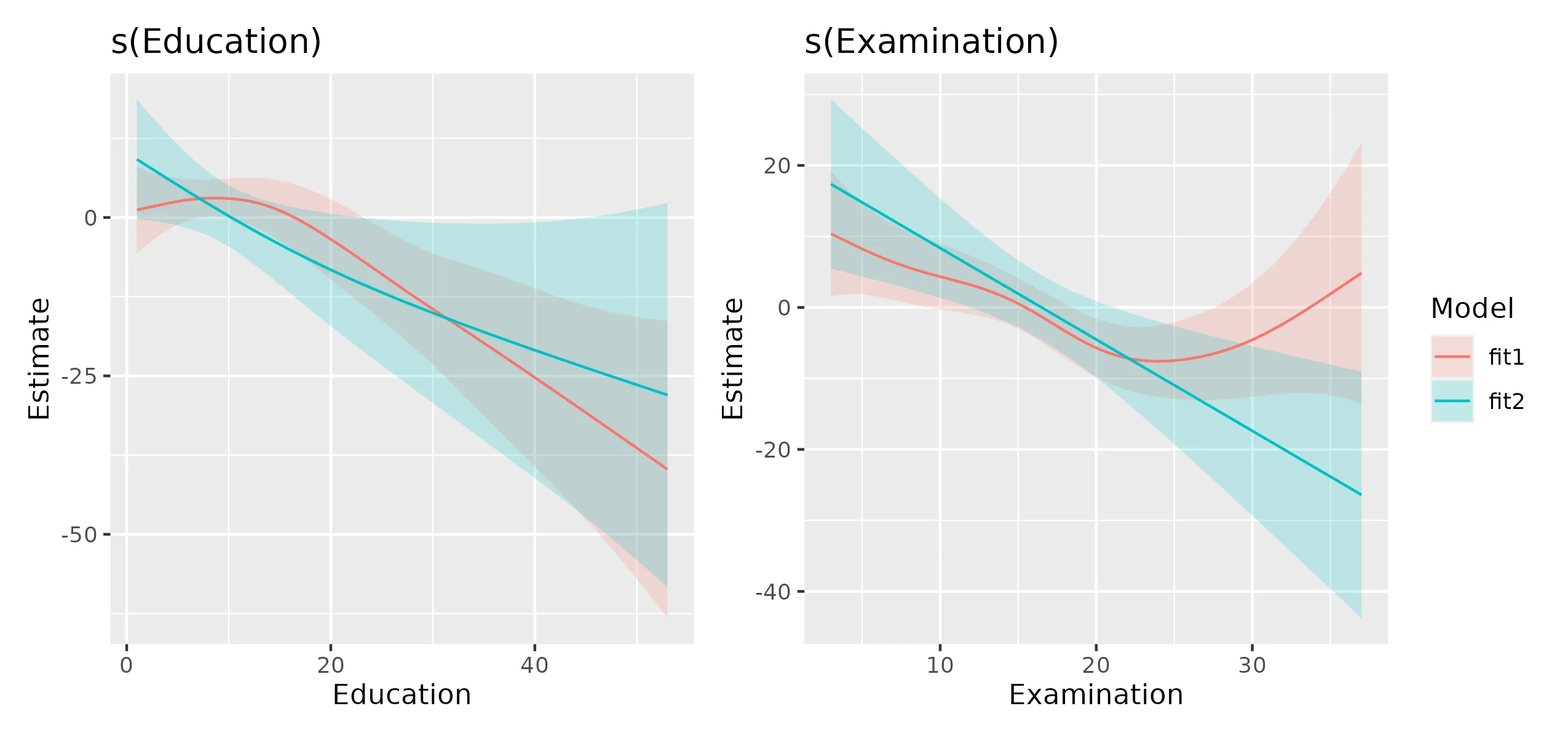
现在使用{patchwork}包将图形放在一起。

library("patchwork")
p_edu + p_exam + plot_layout(guides = "collect")

这会使用{ggplot2}，因此如果您想对颜色有更多控制，需要查看其他比例尺，例如?scale_fill_manual，或者提供其他现成的离散比例尺。

我可以在{gratia}中使其中一些操作更加简单 - 我可以允许用户提供用于颜色和填充的比例尺，如果他们提供原始数据，我还可以画出地毯图。

- Gavin Simpson

---

这是一个非常好而且有用的答案！我只是不确定如何获得图形本身，以更改线条颜色等...我不明白如何从unnest()函数中获取它。我们如何仅获取图形？ - mtao

@mtao 你不能在draw()方法生成的图表上更改颜色等。如果你想要自己制作图表，只要你了解ggplot2，这就非常简单。你是想知道后者怎么做吗？如果是的话，我可以在我的回答中添加一些内容。 - Gavin Simpson

@mtao 完成；添加了一个完整的示例，展示如何修改颜色/填充比例尺并向每个面板添加地毯。 - Gavin Simpson

@mtao 你想在常数项的估计中包含不确定性，还是只是将所有内容向上移动？如果是后者，请在“ucomp”上使用mutate()来添加coef(model)[1L]到est、lower_ci和upper_ci变量。如果你想要前者，那么我建议使用fitted_values()在每个模型上使用相同的数据片段（由data_slice()创建）生成相关的平滑曲线。如果你需要更多帮助，请提出一个新问题，如果你在这里回复，我会看一下。 - Gavin Simpson

谢谢提供信息！我已经创建了一个新的问题，因为我尝试了两个选项，但似乎效果都不太好。这是链接：https://stackoverflow.com/questions/76227580/gam-plots-editing-the-y-axis-to-include-the-intercept-uncertainty - mtao

Answer 2

如果您想将它们绘制在同一张图上，可以使用trt_fit1[["plots"]][[1]]$data$fit从拟合中提取数据并自行绘制。我查看了mgcViz github上的绘图样式。您可以根据需要添加第二个轴或比例尺。

library(tidyverse)
exam_dat <- 
  bind_rows(trt_fit1[["plots"]][[1]]$data$fit %>% mutate(fit = "Fit 1"), 
            trt_fit2[["plots"]][[1]]$data$fit %>% mutate(fit = "Fit 2"))
  

ggplot(data = exam_dat, aes(x = x, y = y, colour = fit)) +
  geom_line() +
  labs(x = "Examination", y = "s(Examination)") + 
  theme_bw() +
  theme(panel.grid.major = element_blank(), panel.grid.minor = element_blank())

如果你想要在同一个面板上显示它们，可以使用gridExtra，因为fit1和fit2都是ggplot对象。

gridExtra::grid.arrange(
  trt_fit1[["plots"]][[2]]$ggObj, 
  trt_fit2[["plots"]][[2]]$ggObj, 
  nrow = 1)

^{2022年02月18日创建，使用 reprex包 (v2.0.1)}

- TrainingPizza

---

有没有关于如何添加GAM的置信区间的想法？我尝试使用“ty”值计算它们，然后+- 2 * se，但似乎效果不佳... - mtao

@mtao 您可以使用作者上面提到的 gratia 包。您可以使用 2*se，但是对于点间隔，它是通过 predict 完成的 (https://stats.stackexchange.com/questions/33327/confidence-interval-for-gam-model)。您还可以通过模拟计算同时置信区间 https://fromthebottomoftheheap.net/2016/12/15/simultaneous-interval-revisited/。 - TrainingPizza